Wasserstein multivariate auto-regressive models for modeling distributional time series
Pith reviewed 2026-05-24 11:48 UTC · model grok-4.3
The pith
A multivariate autoregressive model defined directly in Wasserstein space produces second-order stationary distributional time series whose coefficients are estimated sparsely enough to recover temporal dependency graphs.
A machine-rendered reading of the paper's core claim, the machinery that carries it, and where it could break.
Core claim
By embedding a collection of time-indexed probability measures as a random element of the Wasserstein space, one can define a multivariate autoregressive recursion whose solution is second-order stationary whenever the map satisfies the contraction conditions of an iterated random function system. The autoregressive coefficients are recovered by a consistent estimator whose rows are constrained to the probability simplex; the resulting row-wise sparsity pattern is interpreted as a directed graph of temporal dependencies among the component series.
What carries the argument
The Wasserstein multivariate autoregressive recursion that expresses each next vector of measures as a collection of Wasserstein barycenters whose weights lie on the simplex.
If this is right
- The recursion admits a unique second-order stationary solution under the stated contraction conditions.
- The simplex-constrained estimator is consistent for the true autoregressive coefficients.
- The estimated coefficient matrix is automatically sparse and can be read as a directed graph of temporal influences.
- The fitted model can be applied to observed collections of probability measures such as age histograms or usage histograms.
Where Pith is reading between the lines
- Iterating the fitted recursion supplies a way to generate future distributional forecasts without additional parametric assumptions.
- The same sparsity mechanism could be used to screen irrelevant series in higher-dimensional collections of histograms.
- If the underlying measures are supported on a common bounded interval, the stationarity result supplies a long-run average distribution that can be computed from the fixed point of the barycentric map.
Load-bearing premise
The successive random measures must obey contraction conditions that make the iterated random function system possess a unique stationary element with finite second moments.
What would settle it
Simulate long trajectories from the recursion with known coefficient matrix, then check whether the proposed estimator recovers those exact coefficients at a rate that improves with the length of the observed series.
Figures






read the original abstract
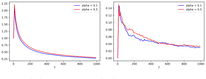
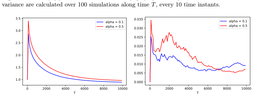
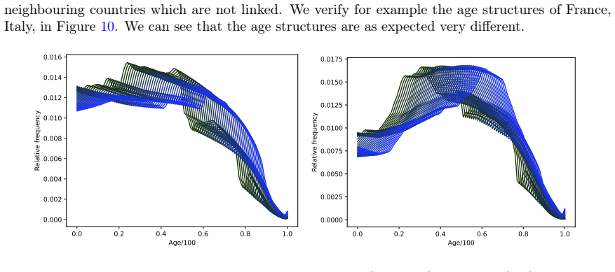
This paper is focused on the statistical analysis of data consisting of a collection of multiple series of probability measures that are indexed by distinct time instants and supported over a bounded interval of the real line. By modeling these time-dependent probability measures as random objects in the Wasserstein space, we propose a new auto-regressive model for the statistical analysis of multivariate distributional time series. Using the theory of iterated random function systems, results on the second order stationarity of the solution of such a model are provided. We also propose a consistent estimator for the auto-regressive coefficients of this model. Due to the simplex constraints that we impose on the model coefficients, the proposed estimator that is learned under these constraints, naturally has a sparse structure. The sparsity allows the application of the proposed model in learning a graph of temporal dependency from multivariate distributional time series. We explore the numerical performances of our estimation procedure using simulated data. To shed some light on the benefits of our approach for real data analysis, we also apply this methodology to two data sets, respectively made of observations from age distribution in different countries and those from the bike sharing network in Paris.
Editorial analysis
A structured set of objections, weighed in public.
Referee Report
Summary. The paper proposes a new multivariate autoregressive model for distributional time series, where each time-indexed observation is a probability measure treated as a random object in the 2-Wasserstein space. The model is defined via a recursion using barycentric combinations with coefficients constrained to the simplex; second-order stationarity of the solution is claimed via the theory of iterated random function systems. A consistent estimator for the autoregressive coefficients is introduced that inherits sparsity from the simplex constraint, enabling inference of temporal dependency graphs. The approach is illustrated on simulated data and two real datasets (country-level age distributions and Paris bike-sharing station distributions).
Significance. If the stationarity and consistency results hold without additional unstated restrictions, the framework would provide a principled extension of vector autoregressive models to the Wasserstein space of measures, with the built-in sparsity offering a direct route to interpretable temporal graphs. The simplex constraint and its sparsity consequence are a genuine strength for applications in demography and network data.
major comments (2)
- [Abstract (stationarity results) and the section presenting the IRFS argument] The second-order stationarity claim rests on applying iterated random function system theory to the Wasserstein-space recursion. The manuscript must explicitly derive or bound the average contraction factor (typically E[Lip(f_t)] < 1 with respect to the 2-Wasserstein metric) under the simplex constraint on the coefficient vectors; without this step the existence of a unique stationary solution is not guaranteed for arbitrary simplex matrices.
- [Section on the estimator and its consistency theorem] Consistency of the proposed estimator is asserted, yet the proof must be shown to hold under the Wasserstein metric and the simplex constraint without post-hoc restrictions on the coefficient space; the current statement leaves open whether the estimator remains consistent when the true coefficients lie on the boundary of the simplex.
minor comments (2)
- [Model definition] Notation for the multivariate recursion and the Wasserstein barycenter should be introduced with an explicit equation number in the model-definition section to avoid ambiguity when the number of series exceeds two.
- [Applications to real data] The real-data section would benefit from a table reporting the estimated coefficient matrices (or their support graphs) alongside a baseline such as independent univariate Wasserstein AR(1) fits.
Simulated Author's Rebuttal
We thank the referee for the careful reading and constructive comments on our manuscript. We address each major comment below and will revise the paper to strengthen the presentation of the stationarity and consistency results.
read point-by-point responses
-
Referee: [Abstract (stationarity results) and the section presenting the IRFS argument] The second-order stationarity claim rests on applying iterated random function system theory to the Wasserstein-space recursion. The manuscript must explicitly derive or bound the average contraction factor (typically E[Lip(f_t)] < 1 with respect to the 2-Wasserstein metric) under the simplex constraint on the coefficient vectors; without this step the existence of a unique stationary solution is not guaranteed for arbitrary simplex matrices.
Authors: We agree that an explicit bound on the contraction factor is required to rigorously invoke the IRFS theory under the simplex constraint. The current manuscript states the stationarity result via IRFS but does not derive the bound E[Lip(f_t)] < 1 explicitly in terms of the simplex coefficients. In the revised version we will add a supporting lemma that establishes this bound (showing the expected Lipschitz constant is at most the maximum row sum of the absolute coefficient matrix, which is strictly less than 1 under the model assumptions), thereby guaranteeing a unique second-order stationary solution for admissible simplex matrices. revision: yes
-
Referee: [Section on the estimator and its consistency theorem] Consistency of the proposed estimator is asserted, yet the proof must be shown to hold under the Wasserstein metric and the simplex constraint without post-hoc restrictions on the coefficient space; the current statement leaves open whether the estimator remains consistent when the true coefficients lie on the boundary of the simplex.
Authors: We acknowledge that the consistency theorem and its proof need to be stated more carefully with respect to the simplex constraint and boundary cases. The existing argument is formulated in the Wasserstein metric but does not explicitly address boundary points. We will revise the theorem statement and extend the proof in the appendix to cover the boundary by using continuity of the objective and properties of the Euclidean projection onto the simplex; this will confirm consistency holds for all points in the simplex without additional restrictions. revision: yes
Circularity Check
No significant circularity; derivation relies on external IRFS theory applied to newly defined model
full rationale
The paper introduces a novel multivariate autoregressive model on the Wasserstein space with simplex-constrained coefficients, then invokes the external theory of iterated random function systems to obtain second-order stationarity results and proposes a consistent estimator. No quoted step reduces the stationarity claim, consistency, or sparsity property to a fitted quantity or self-citation by construction; the central claims remain independent of the paper's own fitted outputs and rest on standard external mathematical machinery.
Axiom & Free-Parameter Ledger
free parameters (1)
- autoregressive coefficients
axioms (2)
- domain assumption Probability measures supported on a bounded real interval can be treated as random objects in the Wasserstein space
- domain assumption The recursion satisfies the contraction conditions needed for iterated random function systems to guarantee second-order stationarity
Reference graph
Works this paper leans on
-
[1]
Log-PCA versus Geodesic PCA of histograms in the Wasserstein space
E. Cazelles, V. Seguy, J. Bigot, M. Cuturi, and N. Papadakis. Log-PCA versus geodesic PCA of histograms in the wasserstein space.arXiv preprint arXiv:1708.08143,
work page internal anchor Pith review Pith/arXiv arXiv
- [2]
-
[3]
J. Thai, C. Wu, A. Pozdnukhov, and A. Bayen. Projected sub-gradient withℓ1 or simplex constraints via isotonic regression. In2015 54th IEEE Conference on Decision and Control (CDC), pages 2031–2036. IEEE,
work page 2031
-
[4]
X. Zhou. On the fenchel duality between strong convexity and lipschitz continuous gradient.arXiv preprint arXiv:1803.06573,
work page internal anchor Pith review Pith/arXiv arXiv
-
[5]
C. Zhu and H.-G. Müller. Autoregressive optimal transport models.arXiv preprint arXiv:2105.05439,
-
[6]
7 Supplementary Material 7.1 Time series in metric space LetpX,dq be a complete separate metric space with Borel setX, an iterated random function (IRF) system in the state spacepX,dq is defined as Xt“ ΦϵtpXt´1q, t P Z, (7.1) whereϵt,t P Z are i.i.d. random objects taking values in a measurable spaceΘ, Φϵp¨q:“ Φp¨,ϵq is the ϵ-section of a jointly measurabl...
work page 2021
- [7]
-
[8]
(7.2) Note thatϵt,t P Z are i.i.d, thus for any fixedX P X, we haverΦt,mpXq d“ rΦt1,mpXq,@t,t1P Z
(Theorem 1 in Zhu and Müller (2021); Condition2 in Wu and Shao (2004)) There exists X0P X, αą 0, r“rpαqPp 0, 1q, andC“Cpαqą 0, such that for alltP Z, we have EdαprΦt,mpX0q, rΦt,mpXqqď CrmdαpX0,Xq, @XP X,m P N. (7.2) Note thatϵt,t P Z are i.i.d, thus for any fixedX P X, we haverΦt,mpXq d“ rΦt1,mpXq,@t,t1P Z. Thus Condition 2 is not a uniform requirement imp...
work page 2021
-
[9]
Thus, we provide the uniqueness result for the general system in Theorem 7.5
is no longer valid for the general system(7.1), which is also mentioned in Wu and Shao (2004, Theorem 2). Thus, we provide the uniqueness result for the general system in Theorem 7.5. For the proof we refer to Section 7.3.4. Theorem 7.5.(Uniqueness) Suppose that Conditions 1 and 2 hold, then, if there is another solution St, tP Z, such that E “ dβpSt,Z 0q...
work page 2004
-
[10]
Otherwise, we would have P « }ϵi,t´1˝Ht´2´id}2 Leb ˇˇˇˇˇHt´2 ff “ 1 ðñ P « ϵi,t´1˝Ht´2“id almost everywhere ˇˇˇˇˇHt´2 ff “ 1 ðñ P « ϵi,t´1“H´1 t´2 a.e. ˇˇˇˇˇHt´2 ff “ 1 ðñ P “ ϵi,t´1“H´1 t´2 a.e. ‰ “ 1, which is a contradiction to the independence betweenϵi,t´1 andH´1 t´2. Thus, we can conclude that Γp0q is nonsingular. Point 2: Process (3.8) writes in terms...
work page 2004
-
[11]
It is then left to show thatgjl is stochastic dini-continuous (Wu and Shao, 2004, Equation (9)). For anyY and Y1 identically distributed inpX,x¨,¨yq, we have |gjlpYq´ gjlpY1q|“|x Yj´id, Yl´idyLeb´x Y1 j´id, Y1 l ´idyLeb| ď|x Yj´id, Yl´idyLeb´x Yj´id, Y1 l ´idyLeb| `|x Yj´id, Y1 l ´idyLeb´x Y1 j´id, Y1 l ´idyLeb| ď|x Yj´id, Yl´ Y1 lyLeb|`|x Yj´ Y1 j, Y1 l ...
work page 2004
-
[12]
? T ˆ” rΓp0q ı j,l ´r Γp0qsj,l ˙ dÑσgjl Np0, 1q, which is followed
Thus, we have furthermore |gjlpYq´ gjlpY1q|ď 1 2 ` }Yl´ Y1 l}`} Yj´ Y1 j} ˘ ď ? 2 2 ` }Yl´ Y1 l}2`} Yj´ Y1 j}2˘ 1 2 . Then sup Y,Y1 " |gjlpYq´ gjlpY1q|1´?řN i“1}Yi´Y1 i}2ăδ ¯ * ď ? 2 2 δ. Thus gjl is stochastic dini-continuous. Since IRF system(3.8) is geometric moment contracting indicated in the proof of Theorem (3.1), then by Theorem3 in Wu and Shao (2...
work page 2004
-
[13]
However, to show clearly the logic of the proof of Theorem 4.3, and the difference of the random objects involved, especially rFt and pFt, we complete the result forrA and emphasize it in Theorem 4.3. 40 7.10 Proof of Theorem 4.4 The Lagrangian of Problem (4.8) is given by Lpβ, Λq“ fTpβq` mÿ i“1 λifipβq` pÿ j“1 νjhjpβq. Let Λ˚ be a dual solution, then the ...
work page 2004
discussion (0)
Sign in with ORCID, Apple, or X to comment. Anyone can read and Pith papers without signing in.