Detection and inference of changes in high-dimensional linear regression with non-sparse structures
Pith reviewed 2026-05-24 03:59 UTC · model grok-4.3
The pith
Exact sparsity of regression parameters or their differences is not needed for consistent multiple change-point detection in high-dimensional linear models.
A machine-rendered reading of the paper's core claim, the machinery that carries it, and where it could break.
Core claim
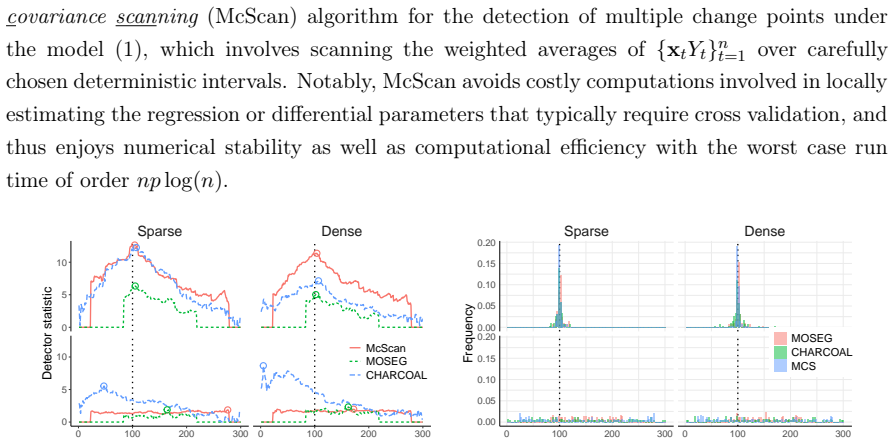
We show that the exact sparsity of neither regression parameters nor their differences is necessary for consistency in multiple change point detection. In fact, both statistically and computationally, better efficiency is attained by a simple strategy that scans for large discrepancies in local covariance between the regressors and the response. We go a step further and propose a suite of tools for directly inferring about the differential parameters post-segmentation, which are applicable even when the regression parameters themselves are non-sparse. Theoretical investigations are conducted under general conditions permitting non-Gaussianity, temporal dependence and ultra-high dimension.
What carries the argument
The covariance-based scan that detects large discrepancies in the local covariance between regressors and response, enabling consistent change-point detection without sparsity assumptions on parameters or differences.
If this is right
- Consistent multiple change-point detection holds without sparsity on either the regression parameters or the differential parameters.
- The covariance scan attains better statistical and computational efficiency than local L1-regularised estimation followed by contrast.
- Inference procedures for differential parameters remain valid after segmentation even when the regression parameters are non-sparse.
- The guarantees extend to non-Gaussian data, temporally dependent observations, and ultra-high-dimensional regressors.
Where Pith is reading between the lines
- The covariance scan may scale more readily to regimes where the number of regressors greatly exceeds sample size per segment.
- Second-moment information alone can suffice for change detection when first-moment parameter estimation is intractable due to lack of sparsity.
- The post-segmentation inference tools could be adapted to test for the presence of changes in specific linear combinations of coefficients.
- Macroeconomic applications may benefit from avoiding sparsity assumptions when regime shifts affect many variables simultaneously.
Load-bearing premise
The stated general conditions on non-Gaussianity, temporal dependence and ultra-high dimensionality suffice for the covariance scan to deliver consistent multiple change-point detection without any sparsity requirement.
What would settle it
A dataset generated under the paper's conditions in which known change points produce no detectable local covariance discrepancies while a sparsity-based estimator still recovers them would falsify the consistency claim.
Figures





read the original abstract
For data segmentation in high-dimensional linear regression settings, the regression parameters are often assumed to be sparse segment-wise, which enables many existing methods to estimate the parameters locally via $\ell_1$-regularised maximum likelihood-type estimation and then contrast them for change point detection. Contrary to this common practice, we show that the exact sparsity of neither regression parameters nor their differences, a.k.a.\ differential parameters, is necessary for consistency in multiple change point detection. In fact, both statistically and computationally, better efficiency is attained by a simple strategy that scans for large discrepancies in local covariance between the regressors and the response. We go a step further and propose a suite of tools for directly inferring about the differential parameters post-segmentation, which are applicable even when the regression parameters themselves are non-sparse. Theoretical investigations are conducted under general conditions permitting non-Gaussianity, temporal dependence and ultra-high dimensionality. Numerical results from simulated and macroeconomic datasets demonstrate the competitiveness and efficacy of the proposed methods. Implementation of all methods is provided in the R package \texttt{inferchange} on GitHub.
Editorial analysis
A structured set of objections, weighed in public.
Referee Report
Summary. The manuscript claims that exact sparsity on the segment-wise regression parameters β or their differences Δβ is unnecessary for consistent multiple change-point detection in high-dimensional linear regression. Instead, a simple covariance scan that detects large discrepancies in the local covariance between regressors and response achieves both statistical and computational efficiency gains. The authors further develop post-segmentation inference procedures for the differential parameters that remain valid even when the β's are dense. Theoretical results are stated under general conditions allowing non-Gaussianity, temporal dependence, and ultra-high dimensionality; numerical evidence is provided on simulated data and macroeconomic series, with an accompanying R package inferchange.
Significance. If the consistency and inference results hold, the work meaningfully relaxes a pervasive sparsity assumption in the change-point literature for high-dimensional regression, replacing it with a directly identifiable covariance discrepancy that targets E[XY] rather than β. This yields both simpler computation and broader applicability to settings where sparsity is implausible. The post-detection inference tools and the open-source implementation are concrete strengths that increase the practical value of the contribution.
minor comments (2)
- The abstract states that the covariance scan attains 'better efficiency' both statistically and computationally, but does not quantify the improvement relative to existing ℓ1-based procedures; a brief comparison of detection thresholds or computational complexity in the introduction would strengthen the claim.
- The package inferchange is mentioned; confirming that the simulation code and macroeconomic data preprocessing scripts are included in the repository would improve reproducibility.
Simulated Author's Rebuttal
We thank the referee for the positive and supportive review, which correctly captures the main contributions of the manuscript. The recommendation for minor revision is appreciated. No specific major comments were raised in the report.
Circularity Check
No significant circularity in derivation chain
full rationale
The paper's central result establishes that exact sparsity on beta or Delta beta is unnecessary for consistent multiple change-point detection, with a covariance scan on local discrepancies in E[X Y] delivering the detection under general conditions permitting non-Gaussianity, temporal dependence and ultra-high dimensionality. This approach directly targets an identifiable quantity without requiring sparse estimation of the regression parameters themselves, and the theoretical support is stated as independent of the sparsity assumption being relaxed. No self-definitional reductions, fitted inputs renamed as predictions, or load-bearing self-citation chains appear in the stated argument; the derivation remains self-contained against external benchmarks.
Axiom & Free-Parameter Ledger
Reference graph
Works this paper leans on
-
[1]
Bai, J. and Perron, P. (1998). Estimating and testing linear models with multiple structural changes. Econometrica, 66(1):47–78. Bai, Y. and Safikhani, A. (2022). A unified framework for change point detection in high- dimensional linear models.arXiv preprint arXiv:2207.09007v1. Baranowski, R., Chen, Y., and Fryzlewicz, P. (2019). Narrowest-over-threshold...
-
[2]
Cai, T. T. and Guo, Z. (2020). Semisupervised inference for explained variance in high dimensional linear regression and its applications.Journal of the Royal Statistical Society Series B: Statistical Methodology, 82(2):391–419. Cai, T. T., Liu, W., and Zhou, H. H. (2016). Estimating sparse precision matrix: Optimal rates of convergence and adaptive estim...
work page internal anchor Pith review Pith/arXiv arXiv 2020
-
[3]
Springer. 30 Javanmard, A. and Montanari, A. (2014). Confidence intervals and hypothesis testing for high-dimensional regression. Journal of Machine Learning Research, 15(1):2869–2909. Kaul, A., Jandhyala, V. K., and Fotopoulos, S. B. (2019). Detection and estimation of param- eters in high dimensional multiple change point regression models viaℓ1/ℓ0 regu...
work page internal anchor Pith review Pith/arXiv arXiv 2014
-
[4]
Xu, H., Wang, D., Zhao, Z., and Yu, Y. (2024). Change-point inference in high-dimensional regression models under temporal dependence.The Annals of Statistics, 52(3):999–1026. Yuan, H., Xi, R., Chen, C., and Deng, M. (2017). Differential network analysis via Lasso penalized D-trace loss.Biometrika, 104(4):755–770. Zhang, C.-H. and Zhang, S. S. (2014). Con...
work page 2024
-
[5]
Recall thatΣ = Cov(xt), δj = βj −βj−1 and ∆j = min(θj −θj−1, θj+1 −θj)
and DPDU (Xu et al., 2024). Recall thatΣ = Cov(xt), δj = βj −βj−1 and ∆j = min(θj −θj−1, θj+1 −θj). We omit the subscriptj as the conditions hold for everyj, and Ψ may depend on n and p. For symmetric matricesA, B ∈ Rp×p, we write A ≲ B to indicate that there is a constant c > 0 such thatx⊤(A − cB)x ≤ 0 for all x ∈ Rp, and A ≍ B if A ≲ B and B ≲ A. Σ β, δ...
work page 2024
-
[6]
Again by the similar calculation as in Part (i), we have α + 1 ≤ exp 2γ κ4 σ4ε + s2 p exp 4γκ2 sσ2ε − 1 = exp κ2 2σ2ε s log 1 + p 17s2 + 1 17 ≤ exp 2 17 < 3 2 , where the last second inequality is due tos log 1 + p/(17s2) ≤ p 2∆/(17τ) and the choice of κ. This concludes the proof. 39 B Multiplier bootstrap Instead of sampling directly from the distributio...
work page 2018
-
[7]
max j′∈{j−1,j} |βj′|2ψn,p s |bθ − θj| ∆◦ . Finally, by (C.8) and Lemma 7 of Wang and Samworth (2018), we have T3 ≥ 2(1 − 8C0/c′) 3 √ 6 |bθ − θ|√ ∆◦ |Σδj|∞. 48 Then, from (C.9), we have 2(1 − 8C0/c′) 3 √ 6 |bθ − θ|√ ∆◦ |Σδj|∞ ≤ C0(2 + √
work page 2018
-
[8]
C.3.2 Supporting lemmas Lemma C.3
1 + max j′∈{j−1,j} |βj′|2 ψn,p s |bθ − θj| ∆◦ , such that |Σδj|2 ∞|bθ − θj| ≤ 3 √ 6(1 + √ 2)C0 1 − 8C0/c′ !2 Ψ2 j ψ2 n,p, from which the conclusion follows with a large enough constantc1. C.3.2 Supporting lemmas Lemma C.3. Suppose that Assumption 2 holds. Then, for all(s, k, e) ∈ I ′ with I ′ = n 0 ≤ s < k < e ≤ n : {s + 1, . . . , e− 1} ∩ Θ ≤ 1 and min(k...
work page 2018
-
[9]
Then, T3 = 1√ bE − aE bE X t=aE+1 wE t ξt
Let ξt = (ξit)i∈[p] := bΩEU◦ t. Then, T3 = 1√ bE − aE bE X t=aE+1 wE t ξt. (C.27) Further, withai = (bΩE i·, 0)⊤ ∈ Rp+1 and b = (( ¯µE)⊤, 1)⊤ ∈ Rp+1, we have ξit = ( bΩEU◦ t )i = a⊤ i ZO t ZO t ⊤ b − E a⊤ i ZO t ZO t ⊤ b DE . Note that |ai|2 ≤ maxi∈[p] |bΩE i·|2 ≤ Λmax bΩE ≤ 3/(2σ) from (C.23), and|b|2 ≤ 1 + |¯µE|2 ≤ Ψj. Then by (C.25) and Lemma C.12, it ...
work page 2018
-
[10]
59 Theabovetailprobabilitybound, togetherwith(C.25), Fubini’stheoremandtheunionbound, implies that (wE t )4E max i∈[p] max aE<t≤bE |ξit|4 DE, QE n,p ≍ Z ∞ 0 P max i∈[p] max aE<t≤bE |ξit|4 ≥ u DE, QE n,p du ≤ Z (2Cξ log(p(bE−aE)))4 0 du + p(bE − aE) Z ∞ (2Cξ log(p(bE−aE)))4 P |ξit|4 ≥ u DE, QE n,p du ≤ 2Cξ log(p(bE − aE)) 4 + 2p(bE − aE) Z ∞ (2Cξ log(p(bE−...
work page 2003
-
[11]
βj−1 + 1 2 bδE j 1 # 2 ≤ 1 + |βj−1|2 + 1 2 |bδE j |2 ≲ 1 + |βj−1|2 + |δj|2,
We frequently use that E E n,p ⊂ S E n,p. The subsequent arguments are conditional onE E n,p ∩ RE n,p ∩ E O n,p ∩eE O n,p with eE O n,p defined in (C.37) below, which fulfilsP(eE O n,p) ≥ 1 − c2(p ∨ n)−c3. Hence, P(E E n,p ∩ RE n,p ∩ E O n,p ∩eE O n,p) ≥ 1 − 4c2(p ∨ n)−c3 by Lemmas C.2 and C.7. By (C.18), which follows from Theorem 2 conditional onE E n,p...
work page 2020
-
[12]
and the union bound, we have P eRc n,p ≤ X 0≤s<e≤n e−s≥CREσ−2ψ2 n,p Cκ exp " −C′ σ√e − s 54Ξ 2 1+2κ + 2bs,e log(p) # ≤ Cκn2 exp − C′ 2 C1/2 RE 54Ξ ! 2 1+2κ log(p ∨ n) , 66 with some constantC′ ∈ (0, ∞) depending only onκ. Here, the last inequality follows with bs,e = $ C′ 4 log(p) σ√e − s 54 2 1+2κ % and the condition on e − s. We can find CRE that...
work page 2012
-
[13]
Next, we consider an orthogonal matrixU ∈ Rp×p such that its first column isδ1/2. In simulation, we generate suchU by applying the Gram–Schmidt orthonormalisation to the collection of δ1 and p − 1 standard normal vectors inRp. Then the observations are generated under the model (1) where we setq = 1, θ1 = 100, n = 300, p = 200, β0 = δ1/2, β1 = −δ1/2 and x...
work page 2024
-
[14]
• VPWBS (Wang et al., 2021): The implementation is provided in the R codes on GitHub (https://github.com/darenwang/VPBS, version of May 26, 2021). We tune the param- eters involved using a cross validation procedure (via the functionvpcusum) provided in the example codes on GitHub. There is no option to set the number of change points. Thus similar to DPD...
work page 2021
-
[15]
and the number of estimated change points, in Figures D.3 to D.5. The V-measure is an entropy-based clustering measure, which takes values in[0, 1] with a larger value indicating a higher accuracy. Unlike the other clustering measures, such as (adjusted) Rand index (Rand, 1971; Hubert and Arabie, 1985), the V-measure satisfies all of the desirable propert...
work page 1971
-
[16]
and γ = 0.9, and varyp ∈ {400, 900} and θ1, θΣ ∈ {75, 150, 225}. (M5) Using the same model parameters as in (M4), we now define Σt = n − t n − 1 · Σ(0)(0.3) + t − 1 n − 1 · Σ(1)(0.3). Setting (n, p, s) = (300, 900, 5), we varyθ1 ∈ {75, 150, 225}. Under (M4), Cov(xt) undergoes an abrupt shift atθΣ, whereas under (M5), it changes grad- ually over time. In b...
work page 2024
-
[17]
For DPDU and VPWBS, we manually select the es- timate nearest to θ1 as described in Section 4.1.1
and VPWBS (Wang et al., 2021), applying all methods with prior knowledge of the number of change points to isolate change point estimation from model selection. For DPDU and VPWBS, we manually select the es- timate nearest to θ1 as described in Section 4.1.1. CHARCOAL (Gao and Wang, 2022a) is excluded since p > n (see Appendix D.2.1 for implementation det...
work page 2021
discussion (0)
Sign in with ORCID, Apple, or X to comment. Anyone can read and Pith papers without signing in.