Bayesian Deep Generative Models for Multiplex Networks with Multiscale Overlapping Clusters
Pith reviewed 2026-05-24 00:45 UTC · model grok-4.3
The pith
A Bayesian hierarchical model infers multiscale overlapping clusters in multiplex networks and proves identifiability plus posterior consistency.
A machine-rendered reading of the paper's core claim, the machinery that carries it, and where it could break.
Core claim
The authors introduce a Bayesian hierarchical generative process whose latent variables encode multiscale overlapping clusters both across the population of networks and within each replicate; they prove identifiability of all parameters via novel technical arguments, establish posterior consistency, and supply efficient posterior computation procedures that recover the population hierarchy and the replicate-specific cluster assignments.
What carries the argument
Bayesian hierarchical generative model with multiscale overlapping clusters defined at both population and replicate levels.
If this is right
- Population-level node hierarchy and replicate-level multi-resolution clusters can be inferred jointly from the same data.
- The identifiability tools apply directly to other hierarchical network models that share similar latent cluster structures.
- Posterior samples yield uncertainty quantification for both the shared hierarchy and the per-network cluster assignments.
- The computation methods scale to real multiplex datasets such as brain connectomes.
Where Pith is reading between the lines
- The same identifiability arguments could be reused to prove consistency for models that add node covariates or edge weights.
- If the model is correct, the inferred population hierarchy supplies a natural way to align clusters across different studies of the same node set.
- The multiscale structure suggests testing whether coarser or finer resolutions dominate prediction error on held-out networks.
Load-bearing premise
The observed networks are produced exactly by the hierarchical generative process that places multiscale overlapping clusters at both the population and the replicate levels.
What would settle it
Generate synthetic multiplex data from the model with known population hierarchy and replicate clusterings, then check whether the posterior sampler recovers those exact structures with high probability as the number of replicates increases.
Figures


read the original abstract
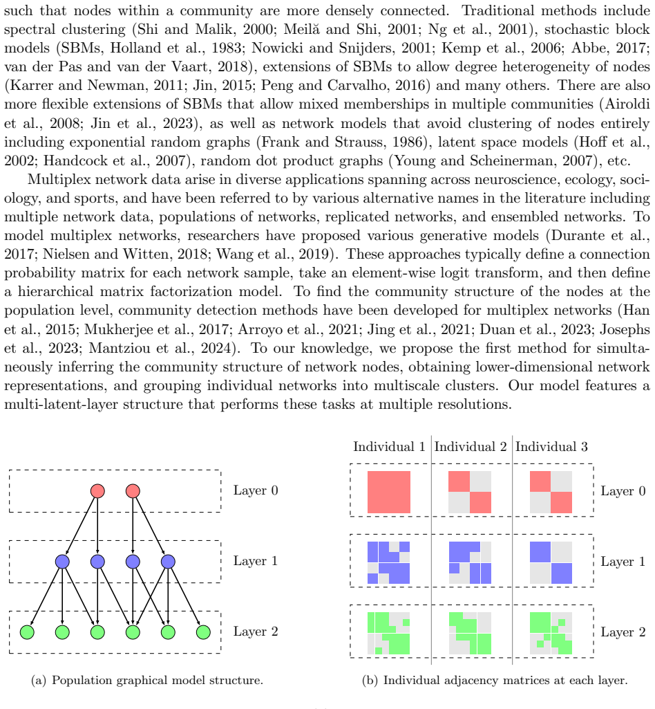
Our interest is in multiplex network data with multiple network samples observed across the same set of nodes. Examples originate from a variety of fields, including brain connectivity, international trade networks, and social networks, among others. Our goal is to infer a hierarchical structure of the nodes at a population level, while performing multi-resolution clustering of the individual replicates. To accomplish this, we propose a Bayesian hierarchical model, provide theoretical support in terms of identifiability and posterior consistency, and design efficient methods for posterior computation. We provide novel technical tools for proving model identifiability, which are of independent interest. Our proposed methodology is demonstrated through numerical simulation and an application to brain connectome data.
Editorial analysis
A structured set of objections, weighed in public.
Referee Report
Summary. The manuscript proposes a Bayesian hierarchical model for multiplex network data observed across multiple samples on the same nodes. The model aims to recover a hierarchical population-level structure on the nodes together with multi-resolution overlapping cluster assignments for the individual replicates. It asserts theoretical support via novel tools establishing model identifiability and posterior consistency, supplies efficient posterior computation methods, and illustrates the approach on numerical simulations and brain connectome data.
Significance. If the identifiability and consistency results can be rigorously established, the work would supply a principled Bayesian framework for multiscale analysis of multiplex networks, addressing overlapping clusters at both population and replicate levels. The claimed novel technical tools for identifiability proofs could be of independent methodological interest beyond the network setting. The brain-connectome application, if accompanied by quantitative validation, would demonstrate practical utility in neuroscience.
major comments (2)
- [Abstract] Abstract: the claims of identifiability, posterior consistency, and efficient computation are asserted without any derivation details, proof sketches, or data-exclusion rules; because these are the central theoretical contributions, the manuscript must supply explicit statements of the assumptions, key steps, and any novel technical tools in a dedicated theory section.
- [Application] Application section: the brain connectome analysis is mentioned without any quantitative results, error bars, or comparison metrics, so it is impossible to assess whether the model recovers meaningful multiscale structure on real data; this demonstration is load-bearing for the practical claim.
minor comments (1)
- [Abstract] The abstract should explicitly reference the section numbers containing the identifiability proofs and the posterior-consistency theorem.
Simulated Author's Rebuttal
We thank the referee for the detailed and constructive report. We address each major comment below and commit to revisions that strengthen the presentation of the theoretical results and the real-data application.
read point-by-point responses
-
Referee: [Abstract] Abstract: the claims of identifiability, posterior consistency, and efficient computation are asserted without any derivation details, proof sketches, or data-exclusion rules; because these are the central theoretical contributions, the manuscript must supply explicit statements of the assumptions, key steps, and any novel technical tools in a dedicated theory section.
Authors: The manuscript already contains a theory section (Section 3) that states the model assumptions, outlines the novel technical tools for identifiability, and provides the key steps and proof sketches for both identifiability and posterior consistency. The abstract is kept concise per standard journal length limits. We will revise the abstract to include a brief, explicit statement of the main assumptions, the novel tools, and the consistency result. We will also add a short subsection in the theory section that consolidates the proof strategy and data-exclusion rules for the consistency theorem. revision: yes
-
Referee: [Application] Application section: the brain connectome analysis is mentioned without any quantitative results, error bars, or comparison metrics, so it is impossible to assess whether the model recovers meaningful multiscale structure on real data; this demonstration is load-bearing for the practical claim.
Authors: We agree that the current application section provides only a qualitative illustration. In the revised manuscript we will add quantitative validation: posterior summaries of the recovered hierarchical structure and multi-resolution clusters with credible intervals, numerical comparison metrics against baseline multiplex clustering methods, and an assessment of alignment with known neuroanatomical partitions. These additions will allow readers to evaluate the practical utility of the model on the connectome data. revision: yes
Circularity Check
No significant circularity
full rationale
The paper proposes a Bayesian hierarchical model for multiplex networks, claiming identifiability and posterior consistency via novel technical tools presented as independent contributions. No load-bearing step is shown to reduce by the paper's own equations to a fitted quantity, self-citation chain, or definitional equivalence; the generative assumption is the standard one required for any such consistency result and does not create internal circularity. The derivation chain is self-contained.
Axiom & Free-Parameter Ledger
axioms (1)
- domain assumption Standard Bayesian hierarchical modeling assumptions including prior distributions on cluster assignments and network edges
invented entities (1)
-
Multiscale overlapping cluster structure
no independent evidence
Forward citations
Cited by 1 Pith paper
-
Beyond Local Independence: High-Dimensional Latent Class Graphical Models with Shared Block Structure
Introduces latent class graphical models with shared block structure for high-dimensional ordinal responses, a three-step estimator, and finite-sample consistency guarantees under high-dimensional scaling.
Reference graph
Works this paper leans on
-
[1]
:=⊙ (i,j)∈I1Λ′ (i,j). Using the formula (⊗c i=1Ci) (⊗c i=1Di) (⊙c i=1Ei) =⊙ c i=1(CiDiEi) for matricesC i,D i,E i of compat- ible dimensions, we obtain Λ′
-
[2]
= 1−λ ⋆ 0 1 ⊗ pk−1 (pk−1 −1) 2 1 0 1 1 ⊗ pk−1 (pk−1 −1) 2 Λ[1],(B.18) whereD ⊗c of a matrixDdenotes the Kronecker product⊗ i∈[c]D. On the right hand side of (B.18), we note that the first term is a upper-triangular square matrix with diagonal all ones and the second term is a lower-triangular square matrix with diagonal all ones, which are both invertible...
-
[3]
is invertible. 36 We define thelexicographical orderbetween any two distinct adjacency matricesX k−1 and eXk−1 asX k−1 ≻lex eXk−1 if and only if there exists (s, t)∈ ⟨p k−1⟩such that Xk−1,s,t > eXk−1,s,t, X k−1,i,j = eXk−1,i,j ∀(i, j)∈ (i, j)∈ ⟨p k−1⟩:i < sor (i=s, j < t) . (B.19) If we vectorize the upper triangular off-diagonal entries (i, j) ofX k−1 in...
-
[4]
is given by (NΛ′ [1])s,t = Y (i,j)∈⟨pk−1⟩ (λ(i,j),1,t −λ ⋆)1X−1 k−1(s)i,j=1 + 1X−1 k−1(s)i,j=0 ,(B.20) whereλ (i,j),1,t denotes the (1, t)th entry ofΛ (i,j). SinceΘ∈ T 0 andA k takes the blockwise form (B.13) withP k =I pk, we have each Γ k,i,j >0 anda k,i =e i fori∈[p k−1], which implies λ(i,j),1,t = exp Ck +a ⊤ k,i(Γk ∗X −1 k−1(t))ak,j 1 + exp Ck +a ⊤ k...
-
[5]
are therefore positive. For 1≤s < t≤ |X k−1|, sinceX −1 k−1(s)≻ lex X−1 k−1(t), there exists (i, j)∈ ⟨p k−1⟩such thatX −1 k−1(s)i,j = 1 andX −1 k−1(t)i,j = 0, which implies (λ(i,j),1,t −λ ⋆)1X−1 k−1(s)i,j=1 + 1X−1 k−1(s)i,j=0 = exp Ck + Γk,i,j X−1 k−1(t)i,j 1 + exp Ck + Γk,i,j X−1 k−1(t)i,j −λ ⋆ = 0. From (B.20), all the upper-triangular off-diagonal entr...
-
[6]
is lower-triangular with positive diagonal entries. This proves thatNΛ ′
-
[7]
With the same procedure, we can also prove that rank K(Λ[2]) =|X k−1|
is invertible, as isΛ [1], and rank K(Λ[1]) =|X k−1|. With the same procedure, we can also prove that rank K(Λ[2]) =|X k−1|. We next show that (Λ[3] ⊙Λ [4])diag(v) has Kruskal rank≥2. Since each column ofΛ [3] ⊙Λ [4] sums to one and each entry ofvis positive byΘ∈ T 0 and our model formulation (2.5), it suffices to show thatΛ [3] ⊙Λ [4] does not have two i...
work page 2009
-
[8]
= exp X1,i,j C′ 1 +a ⊤ 1,i(P0(X0)∗Γ ′ 1)a1,j 1 + exp C′ 1 +a ⊤ 1,i(P0(X0)∗Γ ′ 1)a1,j = exp X1,i,j C1 +a ⊤ 1,i(X0 ∗Γ 1)a1,j 1 + exp C1 +a ⊤ 1,i(X0 ∗Γ 1)a1,j =P(X 1,i,j|X0,A 1,Θ 1). SinceP(P 0(X0)|ν′) =P(X 0|ν) is implied by the definition ofν ′, taking summations we have P(X1|A,Θ ′) = X X0∈X0 P(P(X0)|ν′) Y (i,j)∈⟨p1⟩ P(X1,i,j|P(X0),A 1,Θ ′ 1) = X X0...
work page 2015
-
[9]
See Section B.1 for the definition of Kruskal rank
This also implies rank(M)≥3, since the rank is never small than the Kruskal rank. See Section B.1 for the definition of Kruskal rank. Proof.The cased= 3 follows since all matrices inM 3 are invertible. We prove ford≥4 by contradiction. Suppose there exists distinct indicesi, j, k∈[d] such that the columnsm i,m j,m k ofM∈ M d are linearly dependent, i.e. a...
work page 1965
-
[10]
In the SCORE step, for the topepeigenvectorsξ 1, . . . ,ξ epofY, we divideξ 2, . . . ,ξ epentrywise overξ 1 and stack the resultedep−1 vectors by columns into a matrixR∈R p×ep−1. For intuition purposes, we also consider the matrix eRobtained by applying this SCORE step to E[Y|D,Π,Z] instead ofY, since the difference betweenRand eRis proven to be small. It...
-
[11]
This allows us to find out the pure nodes of the model
In the vertex hunting step, we identify the vertices of this simplex using existing methods such as successive projection (Ara´ ujo et al., 2001; Nascimento and Dias, 2005). This allows us to find out the pure nodes of the model. To improve the robustness of this step, it is often helpful to conductk-means clustering of the rows inRbefore finding the vert...
work page 2001
-
[12]
In the membership reconstruction step, given the pure nodes, the mixed memberships of each node can be recovered through solving linear equation systems. The mixed membershipsΠcan be exactly recovered when the Mixed-SCORE algorithm is applied toE[Y|D,Π,Z]. In practice, onlyYis known and the Mixed-SCORE algorithm is applied toY, but the estimator ofΠobtain...
work page 2015
-
[13]
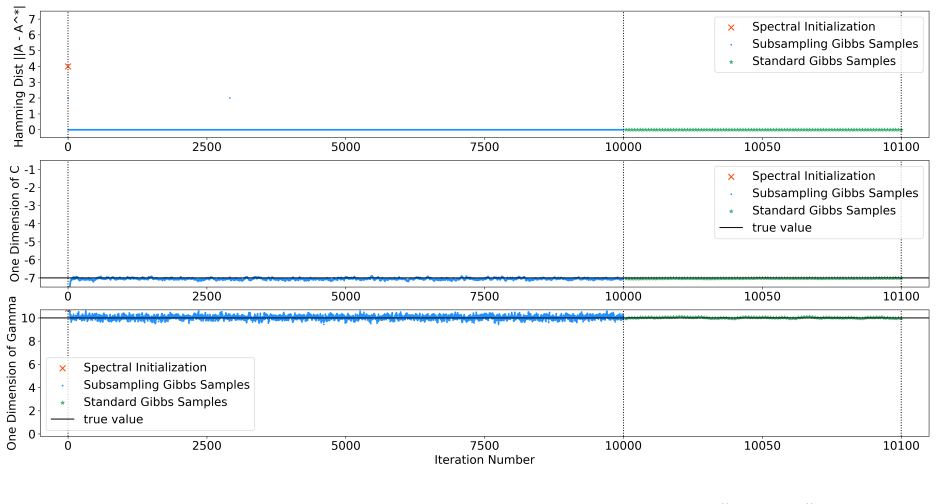
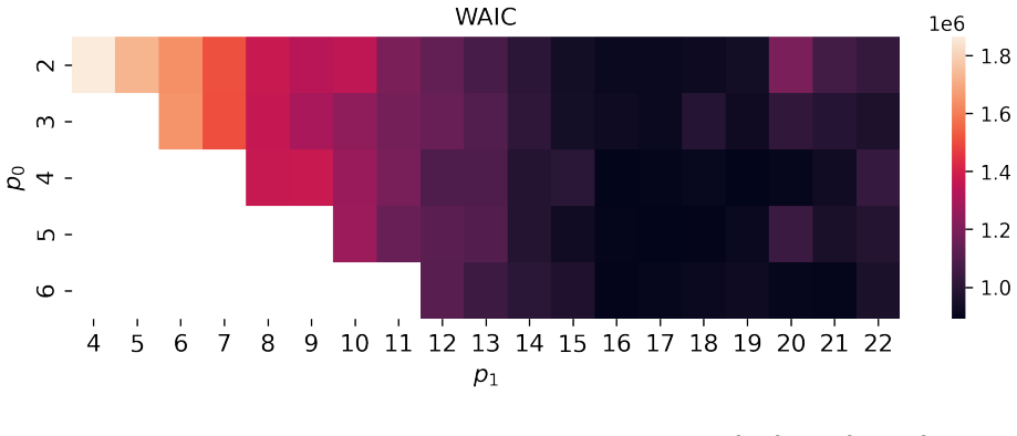
and the Geweke statistic (Geweke, 1992) for convergence diagnosis of both the subsampling and the standard Gibbs samplers. Detailed results reported in Section H.2 provide evidence that the Markov chains of Gibbs samplers under each choice ofp k have converged. Given a Bayesian network structure specified byp k, at thetth iteration of the standard Gibbs s...
work page 1992
-
[14]
This represents a fully-connected ternary tree with its root node removed: the 27 nodes at the finest level are partitioned into 9 leaf communities of size 3, and these leaf communities are further grouped into 3 coarser communities of size 9. LetC (2) 1 , . . . ,C(2) 9 denote the 9 leaf communities of size 3, and letC (1) 1 , . . . ,C(1) 3 denote the coa...
work page 2022
-
[15]
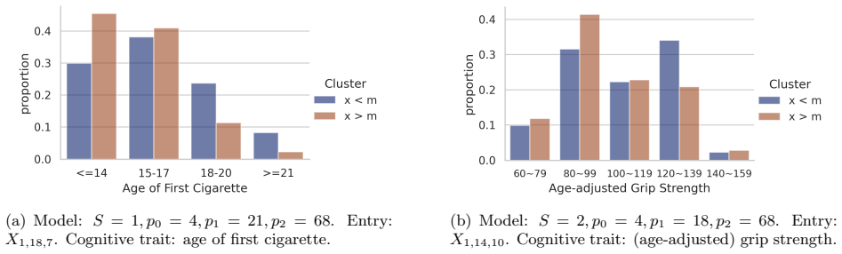
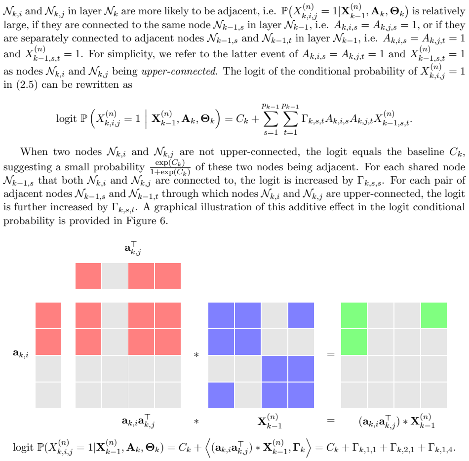
between the latent features and the grouped cognitive measures, with results summarized in Table 3. Second, to assess the practical predictive value of the latent representations, we fit ridge regression models that use the latent features to forecast individual cognitive measures, tuning the regularization parameter by 10-fold cross validation and evalua...
work page 2023
discussion (0)
Sign in with ORCID, Apple, or X to comment. Anyone can read and Pith papers without signing in.