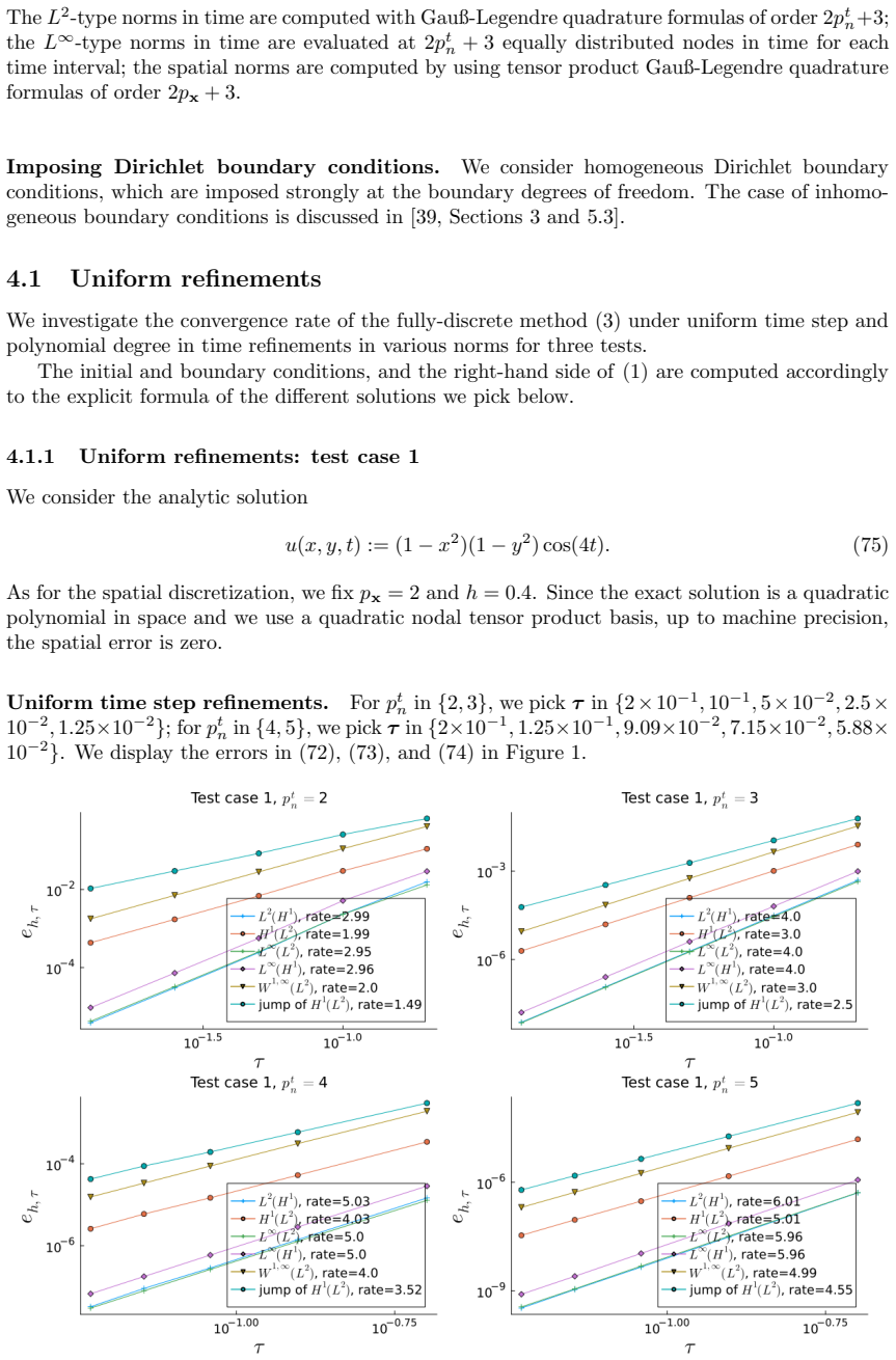
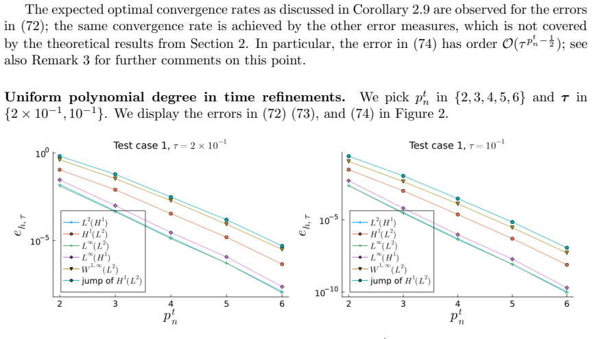
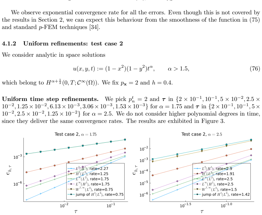
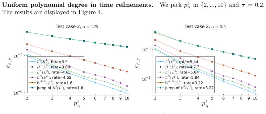
A priori and a posteriori error estimates of a mathcal C⁰-in-time method for the wave equation in second order formulation
Pith reviewed 2026-05-23 17:49 UTC · model grok-4.3
The pith
A discontinuous-continuous Galerkin method yields explicit a priori and a posteriori error estimates for the wave equation.
A machine-rendered reading of the paper's core claim, the machinery that carries it, and where it could break.
Core claim
We establish fully-discrete a priori and semi-discrete in time a posteriori error estimates for a discontinuous-continuous Galerkin discretization of the wave equation; the method uses piecewise polynomial test functions and continuous piecewise polynomial trial functions in time. A priori estimates in L^infty-type norms follow from designed projection operators and nonstandard stability estimates. Reliable a posteriori estimates in L^infty(L^2) with explicit constants are obtained via a reconstruction operator into C^1 piecewise polynomials.
What carries the argument
Discontinuous-continuous Galerkin scheme as a Petrov-Galerkin method with discontinuous test and continuous trial functions in time, supported by projection operators and a C^1 reconstruction operator.
Load-bearing premise
The projection and interpolation operators from the parabolic case extend to the wave equation and the stability estimates based on a nonstandard test function hold.
What would settle it
Numerical computation showing that the a posteriori error estimator fails to bound the true L^infty(L^2) error by the predicted constant, or that a priori estimates do not hold for the chosen operators.
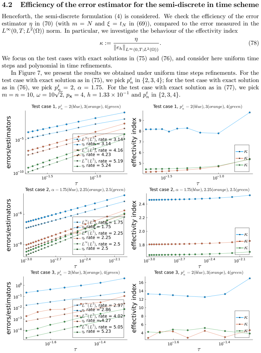
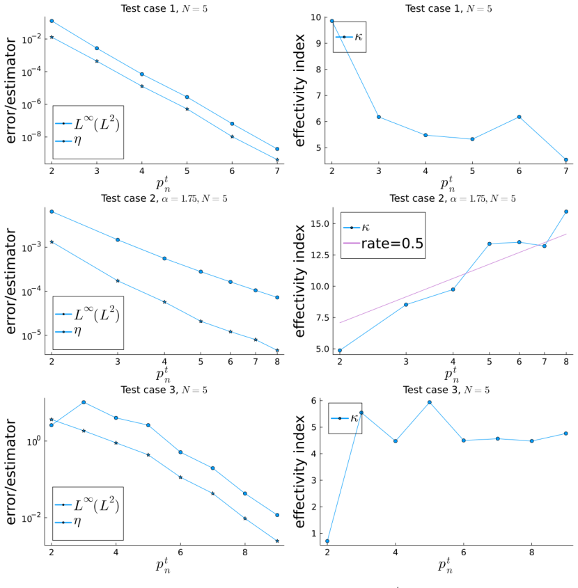
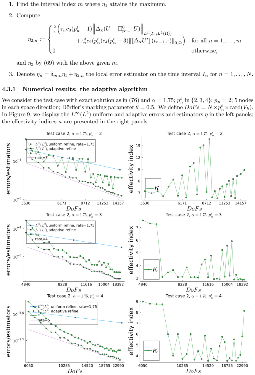
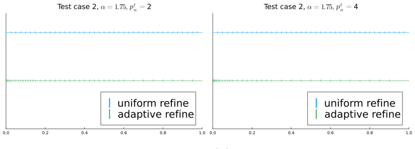
Figures


read the original abstract
We establish fully-discrete a priori and semi-discrete in time a posteriori error estimates for a discontinuous-continuous Galerkin discretization of the wave equation in second order formulation; the resulting method is a Petrov-Galerkin scheme based on piecewise polynomial test functions and continuous piecewise polynomial trial functions in time, respectively. Crucial tools in the a priori analysis for the fully-discrete formulation are the design of suitable projection and interpolation operators extending those used in the parabolic setting, and stability estimates based on a nonstandard choice of the test function; a priori estimates are shown, which are measured in $L^\infty$-type norms in time. For the semi-discrete in time formulation, we exhibit reliable a posteriori error estimates for the error measured in the $L^\infty(L^2)$ norm with fully explicit constants; to this aim, we design a reconstruction operator into $\mathcal C^1$ piecewise polynomials over the time grid with optimal approximation properties in terms of the polynomial degree distribution and the time steps. Numerical examples illustrate the theoretical findings.
Editorial analysis
A structured set of objections, weighed in public.
Referee Report
Summary. The manuscript develops a Petrov-Galerkin discretization of the wave equation in second-order form that is discontinuous in the test functions and continuous (C^0) in the trial functions in time. It derives fully discrete a priori error estimates in L^∞-type norms via specialized projection/interpolation operators extending parabolic techniques together with stability arguments that employ a nonstandard test function. For the semi-discrete-in-time case it constructs a C^1 reconstruction operator with optimal approximation properties and obtains reliable a posteriori bounds in the L^∞(L²) norm that carry fully explicit constants. Numerical examples are included to illustrate the theory.
Significance. If the claimed estimates hold, the work supplies a concrete extension of projection-based a priori analysis and reconstruction-based a posteriori analysis from parabolic to second-order hyperbolic problems, with the explicit constants constituting a practical advantage for adaptive computations. The approach relies on standard approximation-theory tools plus one nonstandard device for stability; the absence of hidden circularity or parameter fitting in the stated argument is a positive feature.
minor comments (3)
- [Abstract] The abstract states that constants are fully explicit; the manuscript should verify in a dedicated remark or appendix that every constant appearing in the final a posteriori bound is indeed independent of the solution and can be computed from the data of the problem alone.
- Notation for the trial and test spaces (continuous vs. discontinuous in time) and for the reconstruction operator should be introduced once in a preliminary section and used consistently thereafter to avoid repeated re-definition.
- The numerical examples section would benefit from a short table reporting observed convergence rates alongside the theoretically predicted rates for at least two different polynomial-degree distributions.
Simulated Author's Rebuttal
We thank the referee for the careful reading and positive assessment of the manuscript, including the recommendation for minor revision. The report does not list any specific major comments requiring response.
Circularity Check
No significant circularity; derivation self-contained
full rationale
The paper constructs projection/interpolation operators extending parabolic techniques and a reconstruction operator into C^1 polynomials, then proves their approximation properties and uses them with a nonstandard test function to derive a priori L^∞-type bounds and explicit a posteriori L^∞(L²) bounds. These steps rely on standard approximation theory and stability arguments rather than any self-definitional reduction, fitted input renamed as prediction, or load-bearing self-citation chain. The central claims are independent of the target error estimates and do not reduce to inputs by construction.
Axiom & Free-Parameter Ledger
Forward citations
Cited by 1 Pith paper
-
A posteriori error analysis and adaptivity of a space-time finite element method for the wave equation in second order formulation
The authors derive rigorous a posteriori error bounds in the L^∞(L²) norm for an arbitrary-order space-time FEM for the wave equation that supports adaptive mesh modification via temporal reconstructions.
Reference graph
Works this paper leans on
-
[1]
S. Adjerid. A posteriori finite element error estimation for second-order hyperbolic problems.Comput. Methods Appl. Mech. Engrg., 191(41-42):4699–4719, 2002
work page 2002
-
[2]
A. K. Aziz and P. Monk. Continuous finite elements in space and time for the heat equation.Math. Comp., 52(186):255–274, 1989
work page 1989
-
[3]
I. Babuˇ ska and J. Osborn. Analysis of finite element methods for second order boundary value problems using mesh dependent norms.Numer. Math., 34(1):41–62, 1980
work page 1980
-
[4]
G. A. Baker. Error estimates for finite element methods for second order hyperbolic equations.SIAM J. Numer. Anal., 13(4):564–576, 1976
work page 1976
-
[5]
Ch. Bernardi and E. S¨ uli. Time and space adaptivity for the second-order wave equation.Math. Models Methods Appl. Sci., 15(02):199–225, 2005
work page 2005
-
[6]
P. Castillo, B. Cockburn, D. Sch¨ otzau, and Ch. Schwab. Optimal a priori error estimates for thehp-version of the local discontinuous Galerkin method for convection–diffusion problems.Math. Comp., 71(238):455–478, 2002
work page 2002
-
[7]
Th. Chaumont-Frelet. Asymptotically constant-free and polynomial-degree-robust a posteriori estimates for space discretizations of the wave equation.SIAM J. Sci. Comput., 45(4):A1591–A1620, 2023
work page 2023
-
[8]
Th. Chaumont-Frelet and A. Ern. Damped energy-norm a posteriori error estimates for fully discrete approxi- mations of the wave equation usingC 2-reconstructions.ESAIM Math. Model. Numer. Anal., 59(4):1937–1972, 2025
work page 1937
-
[9]
Z. Dong, E. H. Georgoulis, L. Mascotto, and Z. Wang. A posteriori error analysis and adaptivity of a space-time finite element method for the wave equation in second order formulation.http://arxiv.org/abs/2509.08537, 2025
work page internal anchor Pith review Pith/arXiv arXiv 2025
-
[10]
L. C. Evans.Partial Differential Equations, volume 19. American Mathematical Society, 2022
work page 2022
-
[11]
M. Feischl. Inf-sup stability implies quasi-orthogonality.Math. Comp., 91(337):2059–2094, 2022
work page 2059
-
[12]
M. Feischl and D. Niederkofler. Optimal adaptive implicit time stepping.https://arxiv.org/abs/2506.18809, 2025
-
[13]
D. A. French. A space-time finite element method for the wave equation.Comput. Methods Appl. Mech. Engrg., 107(1-2):145–157, 1993
work page 1993
-
[14]
D. A. French and T. E. Peterson. A continuous space-time finite element method for the wave equation.Math. Comp., 65(214):491–506, 1996
work page 1996
-
[15]
E. H. Georgoulis, O. Lakkis, and Ch. Makridakis. A posterioriL ∞(L2)-error bounds for finite element approx- imations to the wave equation.IMA J. Numer. Anal., 33(4):1245–1264, 2013
work page 2013
-
[16]
E. H. Georgoulis, O. Lakkis, Ch. Makridakis, and J. M. Virtanen. A posteriori error estimates for leap-frog and cosine methods for second order evolution problems.SIAM J. Numer. Anal., 54(1):120–136, 2016
work page 2016
-
[17]
E. H. Georgoulis, O. Lakkis, and Th. P. Wihler. A posteriori error bounds for fully-discretehp-discontinuous Galerkin timestepping methods for parabolic problems.Numer. Math., 148:363–386, 2021
work page 2021
-
[18]
S. G´ omez and V. Nikoliˇ c. Combined DG–CG finite element method for the Westervelt equation.IMA J. Numer. Anal., page draf080, 09 2025
work page 2025
-
[19]
O. Gorynina, A. Lozinski, and M. Picasso. Time and space adaptivity of the wave equation discretized in time by a second-order scheme.IMA J. Numer. Anal., 39(4):1672–1705, 2019
work page 2019
-
[20]
Grisvard.Elliptic Problems in Nonsmooth Domains, volume 69 ofClassics in Applied Mathematics
P. Grisvard.Elliptic Problems in Nonsmooth Domains, volume 69 ofClassics in Applied Mathematics. SIAM, 2011
work page 2011
- [21]
-
[22]
B. Holm and Th. P. Wihler. Continuous and discontinuous Galerkin time stepping methods for nonlinear initial value problems with application to finite time blow-up.Numer. Math., 138(3):767–799, 2018
work page 2018
-
[23]
G. M. Hulbert and Th. J. R. Hughes. Space-time finite element methods for second-order hyperbolic equations. Comput. Methods Appl. Mech. Engrg., 84(3):327–348, 1990
work page 1990
- [24]
-
[25]
C. Johnson. Discontinuous Galerkin finite element methods for second order hyperbolic problems.Comput. Methods Appl. Mech. Engrg., 107(1-2):117–129, 1993
work page 1993
-
[26]
O. Karakashian and Ch. Makridakis. Convergence of a continuous Galerkin method with mesh modification for nonlinear wave equations.Math. Comp., 74(249):85–102, 2005
work page 2005
-
[27]
Ch. Makridakis and R. H. Nochetto. A posteriori error analysis for higher order dissipative methods for evolution problems.Numer. Math., 104(4):489–514, 2006. 34
work page 2006
-
[28]
Ch. G. Makridakis. On the Babuˇ ska-Osborn approach to finite element analysis:L2 estimates for unstructured meshes.Numer. Math., 139(4):831–844, 2018
work page 2018
-
[29]
F. M¨ uller, D. Sch¨ otzau, and Ch. Schwab. Symmetric interior penalty discontinuous Galerkin methods for elliptic problems in polygons.SIAM J. Numer. Anal., 55(5):2490–2521, 2017
work page 2017
-
[30]
N. Nataraj, R. Ruiz-Baier, and A. Yousuf. Semi and fully-discrete analysis of lowest-order nonstandard finite element methods for the biharmonic wave problem.Comput. Methods Appl. Math., 25(4):921–948, 2025
work page 2025
-
[31]
P.-A. Raviart and J.-M. Thomas.Introduction ` a l’analyse num´ erique des ´ equations aux d´ eriv´ ees partielles. Collection Math´ ematiques Appliqu´ ees pour la Maˆ ıtrise. [Collection of Applied Mathematics for the Master’s Degree]. Masson, Paris, 1983
work page 1983
-
[32]
D. Sch¨ otzau and Ch. Schwab. Time discretization of parabolic problems by thehp-version of the discontinuous Galerkin finite element method.SIAM J. Numer. Anal., 38(3):837–875, 2000
work page 2000
-
[33]
D. Sch¨ otzau and Th. P. Wihler. A posteriori error estimation forhp-version time-stepping methods for parabolic partial differential equations.Numer. Math., 115(3):475–509, 2010
work page 2010
-
[34]
Schwab.p- andhp-Finite Element Methods: Theory and Applications in Solid and Fluid Mechanics
Ch. Schwab.p- andhp-Finite Element Methods: Theory and Applications in Solid and Fluid Mechanics. The Clarendon Press, Oxford University Press, New York, 1998
work page 1998
-
[35]
E. S¨ uli. A posteriori error analysis and adaptivity for finite element approximations of hyperbolic problems. In An Introduction to Recent Developments in Theory and Numerics for Conservation Laws: Proceedings of the International School on Theory and Numerics for Conservation Laws, Freiburg/Littenweiler, October 20–24, 1997, pages 123–194. Springer, 1999
work page 1997
-
[36]
Thom´ ee.Galerkin Finite Element Methods for Parabolic Problems, volume 25
V. Thom´ ee.Galerkin Finite Element Methods for Parabolic Problems, volume 25. Springer Science & Business Media, 2007
work page 2007
-
[37]
L. N. Trefethen.Approximation Theory and Approximation Practice, Extended Edition. Society for Industrial and Applied Mathematics, Philadelphia, PA, 2019
work page 2019
-
[38]
F. Verdugo and S. Badia. The software design of Gridap: a finite element package based on the Julia JIT compiler.Comput. Phys. Commun., 276:Paper No. 108341, 24, 2022
work page 2022
-
[39]
N. J. Walkington. Combined DG–CG time stepping for wave equations.SIAM J. Numer. Anal., 52(3):1398– 1417, 2014. 35
work page 2014
discussion (0)
Sign in with ORCID, Apple, or X to comment. Anyone can read and Pith papers without signing in.