REVIEW 4 major objections 6 minor 7 references
Application of signal separation to diffraction image compression and serial crystallography
T0 review · 4 major / 6 minor · reviewed 2026-08-12 · deepseek-v4-flash
Pith's one-line read Iterative sigma-clipping in azimuthal space separates amorphous background from Bragg peaks and preserves crystallographic data under 2× compression.
desk verdict Solid production-tested beamline software paper with real novelty; fix the variance equations and add error bars before relying on the equivalence claim. read the letter →
The pith
A machine-rendered reading of the paper's core claim, the machinery that carries it, and where it could break.
The reading
What carries the argument
The mechanism is iterative sigma-clipping performed per radial ring in azimuthal space. After dark-current and normalization corrections, each pixel is assigned to a radial bin; the weighted average and variance of the pixel intensities within each bin are computed in a single sparse-matrix multiplication. Pixels whose intensity deviates from the bin average by more than a threshold times the bin standard deviation are flagged and discarded, and the average and variance are recomputed on the remaining pixels until no more outliers are found. The threshold can be set by hand or derived from a Chauvenet-style criterion that adapts to the number of pixels in the ring. The key point is that the per-ring variance is used for clipping rather than a Poissonian error model, which avoids the artifact that bins containing a strong Bragg peak on a low background are emptied entirely. The resulting background curve is a statistically resistant estimate of the amorphous component, and the outlier pixels constitute the Bragg-peak component.
What would settle it
Run the sparsification at 0.8σ on a fixed-target frame whose background is visibly anisotropic (e.g., from a stretched plastic film), densify it, and reduce the structure: if Rfree or the recovered electron density map degrades substantially relative to the isotropic-background case, the central claim is falsified for that sample class.
Extended reading notes
Core claim
The central claim is that iterative sigma-clipping in azimuthal space separates the isotropic amorphous background from Bragg peaks in a single-crystal diffraction image. The paper shows that saving only pixels that deviate from the per-ring background estimate by more than a chosen number of standard deviations, together with a compact description of the background curve and its uncertainty, yields a lossy compression that leaves crystallographic quality indicators nearly unchanged: a cut-off at 0.8 standard deviations gives roughly a twofold compression on photon-counting detector data, and a cut-off at 1.0 standard deviations around 2.6-fold, while the reconstructed electron density map of a test protein is hardly distinguishable from the original. The same background estimate drives a peak-finder that locates Bragg spots at GPU speeds and, when used as a frame veto, can discard a third of the frames from a serial crystallography run while losing only 0.16% of indexable frames.
Load-bearing premise
The background signal must be isotropic, smoothly varying, and far more numerous than the peaks, as the paper explicitly states; anisotropic backgrounds such as those from stretched plastic films in fixed-target mode are outside the method's scope.
Editorial extensions
If this is right
- A sparsification threshold of 0.8 standard deviations yields a 2–3× compression on serial crystallography data while preserving Rfree and the electron density map.
- At a 1.0σ threshold, a protein structure can still be refined with very limited degradation of Rfree and CC1/2, giving users a tunable trade-off between storage and signal preservation.
- The same per-ring background estimate powers a peak-finder whose indexing rate is on par with established methods but runs in milliseconds per frame on a GPU, enabling online vetoing.
- Using the count of picked peaks as a frame veto can save about one third of disk space and bandwidth in a serial crystallography experiment while losing only 0.16% of indexable frames.
- Because background extraction, sparsification, and peak-picking all come from one pass over the image, the pipeline can be embedded in a real-time acquisition loop without reading frames twice.
Reading between the lines
- If the isotropic-background assumption holds for powder diffraction with weak preferred orientation, the same separation could support powder indexing or texture analysis, a use the paper does not test.
- The sparsification scheme could be combined with lossy compressors tuned for smooth backgrounds, potentially pushing effective compression beyond the sigma-threshold bound on datasets where peaks are sparse.
- The per-ring variance statistics could be reused as a physically grounded signal-to-noise map for machine-learning-based frame classification, without additional computation.
- A natural extension would be to test sparsification thresholds below 0.8σ on weak anomalous scatterers, since the paper only reports thresholds from 0.8σ upward.
Signed reviews
Editorial analysis
A structured set of objections, weighed in public.
Referee Report
Summary. The paper presents a signal-separation algorithm based on iterative sigma-clipping in azimuthal space to decompose diffraction images into an isotropic background and Bragg-peak outliers, and applies it to two tasks: lossy compression (sparsification) and peak-finding for serial crystallography. The authors validate the approach on Eiger and Jungfrau detector data using external reduction packages (XDS, CrystFEL, xgandalf, peakfinder8/9), reporting compression ratios of 2–5× with apparent limited degradation of crystallographic quality indicators, and peak-finding performance comparable to established algorithms at lower computational cost. The central claims are that sparsification at 0.8–1.0σ preserves structure-solution quality and that the pyFAI peak-finder achieves indexing rates in line with reference implementations.
Significance. If the claims hold, the work is practically significant for high-frame-rate serial crystallography: it offers a real-time path to reduce bandwidth and storage for detectors like Jungfrau 4M, and it provides an online veto mechanism based on peak counts. The paper's strengths include independent validation against established software (XDS, CrystFEL, xgandalf, peakfinder8/9), an open-source implementation, and an honest discussion of limitations (isotropic-background assumption, detector-geometry sensitivity in Section 4.4). The main weakness is statistical: the key equivalence and parity claims are supported only by single point estimates without uncertainty quantification, and one variance-propagation formula is not derived and is potentially incorrect.
major comments (4)
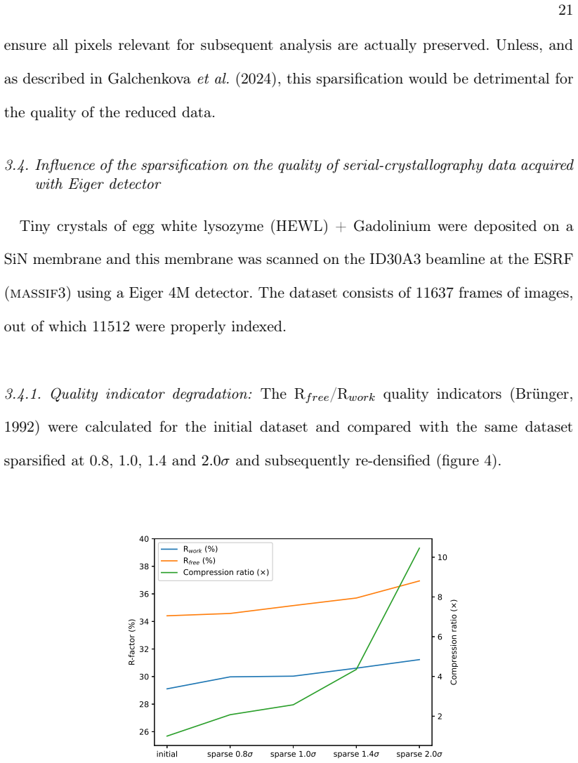
- [Section 3.4–3.6, Fig. 4 and Fig. 6] The central claim that a sparsification at 0.8σ is 'hardly distinguishable' from the uncompressed data rests on single point estimates of Rwork/Rfree and placed-residue counts from one dataset of 11,637 frames. No standard errors, confidence intervals, or repeated refinements are reported. For example, Figure 4 shows an Rfree difference of roughly one percentage point between the initial and 0.8σ datasets, which is within the typical noise of crystallographic refinement, and Figure 6 shows a difference of a few residues that is not statistically meaningful. The authors should provide uncertainty estimates (e.g., via split-half or bootstrap resampling of the 11,512 indexed frames) or soften the equivalence claim.
- [Section 4.2, Table 3] The indexing-rate comparison in Table 3 (49.7% for pyFAI vs 49.5% for PeakFinder8 over 1,000 frames) has a binomial standard error of about 1.6 percentage points, so the difference is not statistically significant. The statement that pyFAI is 'in par' with peakfinder8 is therefore not quantitatively established by these numbers, although the runtime comparison in Section 4.1 clearly shows a computational advantage. The authors should report confidence intervals for the indexing rates or explicitly acknowledge that the rates are statistically indistinguishable.
- [Section 2.2.3, Eq. (4)] The variance-propagation formula in Eq. (4) is not derived and appears inconsistent with standard error propagation for a weighted mean. For a weighted average M = (∑ c_i norm_i v_i)/(∑ c_i norm_i), the variance of M is (∑ c_i² norm_i² σ_i²)/(∑ c_i norm_i)², with a squared denominator, whereas Eq. (4) contains only a single power of (∑ c_i norm_i). If Eq. (4) is intended to give the standard deviation of pixel values rather than the standard error of the mean, the text should state this explicitly and justify the weighting scheme (c_i² in the numerator, c_i norm_i in the denominator). As written, the formula is likely to mislead readers who use it for error propagation.
- [Section 3.5–3.6] The claim that a sparsification at 0.8σ gives a 2.6× compression on Jungfrau data is not directly supported by the tables or figures in Section 3.5: Table 2 reports compression ratios for dense, 1.0σ, and 1.4σ only (3.2× and 5.2× respectively), and no 0.8σ results are shown for the NQO1 dataset. The 2.6× figure appears to be an interpolation or an unreported analysis. Please either cite the specific figure/table that contains the 0.8σ Jungfrau results or present them explicitly.
minor comments (6)
- [Section 1.1] The spelling 'perfom' in the sentence 'require modifications to the experimental setup to perfom SSX experiments' should be corrected to 'perform'.
- [Section 3.3.1] The term 'Poissonnian' appears in the text; the standard spelling is 'Poissonian'.
- [Section 3.3.1] The phrase 'instead of the 5000GB of the original files compressed in LZ4' is likely a typo; the size of the original compressed dataset is probably 5000 MB or 5 GB, not 5000 GB.
- [Section 3.3.4] In the sentence 'Those integrator are measured on integral peaks', the word 'integrator' should be 'indicators'.
- [Section 4.2, Table 3 caption] The run-times reported in Table 3 include both peak finding and indexing, but the text in Section 4.1 reports peak-finding times separately. Please clarify in the caption or text that the run-times in Table 3 are not the peak-finding times alone, to avoid confusion.
- [Section 3.6] The phrase 'preserves nicely the electron density map' is vague; please quantify the preservation with a specific metric such as map correlation or phase error, ideally with confidence intervals.
Circularity Check
No significant circularity: the central claims are validated against external programs and explicit threshold sweeps, not by construction or by load-bearing self-citation.
full rationale
The paper's main claims are the sparsification compression scheme and the pyFAI peak-finder. Neither reduces to its own inputs. The sparsification quality is assessed by processing dense and sparsified datasets with external crystallographic packages (XDS for the Eiger dataset, CrystFEL with xgandalf for the Jungfrau dataset) and comparing Rwork/Rfree, CC1/2, Rsplit, completeness, and automatically placed residues. These metrics are external to the paper's own code and are not fitted parameters. The sparsification threshold is a user-set parameter that is varied (0.8, 1.0, 1.4, and 2.0 sigma) with reported gradual degradation, so the 'hardly distinguishable at 0.8 sigma' statement is an empirical observation from that sweep rather than a quantity forced by definition. The peak-finder is compared with peakfinder8, peakfinder9, zaef, and RobustPF through indexing rates obtained with xgandalf, an independent indexer. The only parameter equalization is explicitly acknowledged in Section 4.1 ('Those parameters have been tuned to obtain a comparable number of peaks with both implementations'), and it affects total peak counts, not the subsequent spatial-distribution comparison. Self-citations to pyFAI, LImA2, and Debionne et al. are implementation provenance and prior code, not a uniqueness theorem or a hidden premise imported from the authors. The stated limitations, such as the isotropic-background requirement in Section 2.3 and the Jungfrau geometry/mask misalignment in Section 4.4, are honest boundary conditions rather than circular steps. The reviewer-level concern about single-point estimates and lack of error bars is a statistical precision issue, not a circularity issue.
Assumptions & free parameters
free parameters (3)
- Picking cut-off n (SNR_pick) =
tested at 0.8, 1.0, 1.4, 2.0; 1.5 needed for 6.4x on ID29
- Peak-finding SNR threshold =
3 in Section 4.1, 5 in Section 4.2
- Local peak patch size =
3x3 or 5x5
assumptions (4)
- domain assumption Background scattering from amorphous or powder material is isotropic and slowly varying in azimuth.
- domain assumption After sigma-clipping, the remaining pixel intensities in each radial bin follow a normal distribution.
- domain assumption The detector signal is described by Poisson counting statistics plus dark-current noise for variance propagation.
- domain assumption Detector geometry and pixel mask descriptions are accurate enough for peak positions to index.
Cite this review
Pith. "Pith review of Application of signal separation to diffraction image compression and serial crystallography." pith.science (2026). https://pith.science/paper/2BA72GCP
@misc{pith2026241109515,
  author       = {Pith},
  title        = {Pith review of: Application of signal separation to diffraction image compression and serial crystallography},
  year         = {2026},
  howpublished = {\url{https://pith.science/paper/2BA72GCP}},
  note         = {Machine review of arXiv:2411.09515}
}
read the original abstract
We present here a real-time analysis of diffraction images acquired at high frame-rate (925 Hz) and its application to macromolecular serial crystallography. The software uses a new signal separation algorithm, able to distinguish the amorphous (or powder diffraction) component from the diffraction signal originating from single crystals. It relies on the ability to work efficiently in azimuthal space and derives from the work performed on pyFAI, the fast azimuthal integration library. Two applications are built upon this separation algorithm: a lossy compression algorithm and a peak-picking algorithm; the performances of both is assessed by comparing data quality after reduction with XDS and CrystFEL.
Figures


Figures from the paper (9 more)


Reference graph
Works this paper leans on
-
[1]
Afonine, P. V., Grosse-Kunstleve, R. W., Echols, N., Headd, J. J., Moriarty, N. W., Mustyaki- mov, M., Terwilliger, T. C., Urzhumtsev, A., Zwart, P. H. & Ad ams, P. D. (2012). Acta Crystallographica Section D , 68(4), 352–367. https://doi.org/10.1107/S0907444912001308 Barty, A., Kirian, R. A., Maia, F. R. N. C., Hantke, M., Yoon, C . H., White, T. A. & Ch...
arXiv 2012
-
[2]
https://gitlab.esrf.fr/limagroup/lima2 Debionne, S., Homs, A., Claustre, L., Kieffer, J., De Sanctis , D., Santoni, G., Goetz, A. & Meyer, J. (2022 b). In Proceedings of the 14th international conference on Synchrotron Radiation Instrumentation (SRI2021) . https://indico.desy.de/event/27430/abstracts/ Dectris, (2014). https://www.dectris.com/support/downlo...
work page 2014
-
[5]
http://www.hdfgroup.org/HDF5 Toledo, S. (1997). IBM Journal of Research and Development , 41(6), 711–725. IUCr macros version 2.1.15: 2021/03/05 42 Underwood, R., Yoon, C., Gok, A., Di, S. & Cappello, F. (2023) . Synchrotron Radiation News, 36(4), 17–22. https://doi.org/10.1080/08940886.2023.2245722 Vincent, T., Valls, V., Payno, H., Kieffer, J., Solé, V. ...
-
[6]
User-Defined Functions for HDF5
https://doi.org/10.3847/1538-4365/aad23d Mariani, V., Morgan, A., Yoon, C. H., Lane, T. J., White, T. A. , O’Grady, C., Kuhn, M., Aplin, S., Koglin, J., Barty, A. & Chapman, H. N. (2016). Journal of Applied Crystallography , 49(3), 1073–1080. https://doi.org/10.1107/S1600576716007469 Masui, K., Amiri, M., Connor, L., Deng, M., Fandino, M., Höfe r, C., Hal...
work page Pith review arXiv 2016
-
[272]
https://doi.org/10.1007/978-1-4939-7000-1_10 Fang, F., Wang, T., Wu, S
New York, NY: Springer New York. https://doi.org/10.1007/978-1-4939-7000-1_10 Fang, F., Wang, T., Wu, S. & Zhang, G. (2020). Information Sciences , 514, 56–70. https://www.sciencedirect.com/science/article/pii/S0020025519311090 Galchenkova, M., Tolstikova, A., Klopprogge, B., Sprenger , J., Oberthuer, D., Brehm, W., White, T. A., Barty, A., Chapman, H. N....
-
[704]
M., Roedig, P., Kuo, A., Evans, G., Sauter, N
https://doi.org/10.1107/S2053273319010593 Ginn, H. M., Roedig, P., Kuo, A., Evans, G., Sauter, N. K., Ern st, O. P., Meents, A., Mueller- Werkmeister, H., Miller, R. J. D. & Stuart, D. I. (2016). Acta Crystallographica Section D, 72(8), 956–965. https://doi.org/10.1107/S2059798316010706 Grieco, A., Boneta, S., Gavira, J. A., Pey, A. L., Basu, S., Or lans,...
-
[2014]
PyFAI: a Python library for high performance azimuthal integration on GPU
http://arxiv.org/pdf/1412.6367.pdf Kieffer, J., Valls, V., Blanc, N. & Hennig, C. (2020). Journal of Synchrotron Radiation , 27(2), 558–566. https://doi.org/10.1107/S1600577520000776 Kieffer, J. & Wright, J. (2013). Powder Diffraction , 28(S2), S339–S350. Kleinwort, C., (2021-2024). Millepede-ii. https://gitlab.desy.de/claus.kleinwort/millepede-ii Klöckner, ...
work page Pith review arXiv 2020
Reviewed August 12, 2026 · model on record in the stance chip above.
Discussion (0). Continue with ORCID to comment.