REVIEW 3 major objections 6 minor 2 cited by
Adaptive Neural Network Subspace Method for Solving Partial Differential Equations with High Accuracy
T0 review · 3 major / 6 minor · reviewed 2026-08-11 · deepseek-v4-flash
Pith's one-line read A neural-network solver for PDEs reaches high accuracy only when the integrals in its loss are computed accurately, not merely when the network is big.
desk verdict The paper's strongest point is the controlled experiment showing quadrature accuracy, not network architecture, limits neural PDE solvers, and it earns a conditional peer-review pass despite the hand-crafted quadrature and missing baselines. read the letter →
The pith
A machine-rendered reading of the paper's core claim, the machinery that carries it, and where it could break.
The reading
What carries the argument
The central mechanism is the neural-network subspace $V_p := \mathrm{span}\{\varphi_j(x;\theta),\,j=1,\dots,p\}$ built from the outputs of a network, over which a Galerkin or Ritz problem is solved exactly by assembling stiffness matrix and right-hand side; training then updates the parameters $\theta$ by minimizing either the Ritz energy or the a posteriori error estimator $\eta(u_p,y)$ from the hypercircle and complementarity theory, which upper-bounds the energy error. The quadrature rules that carry the argument are Gauss-Jacobi quadrature for singular factors of the form $(x-\tfrac12)^{-2/3}$, composite Gauss-Legendre for regular terms, and composite Gauss-Lobatto on subdomains and interfaces; these make the integration error $\varepsilon_{int}$ negligible for the non-polynomial neural-network integrands. The a posteriori loss also measures the dual error through the identity $\eta^2(\psi,y)=\|u-\psi\|_a^2+\|y^*-y\|_*^2$, so minimizing it drives both the primal and dual approximations.
What would settle it
Use the same subspace training on the singular Laplace problem but with an off-center singularity, say at $x_1=0.37$, and only uniform Gauss-Legendre quadrature; if the relative test error does not approach the 1e-5 level as the number of quadrature points grows, the paper's claim that integration accuracy is the controlling factor would be falsified.
Extended reading notes
Core claim
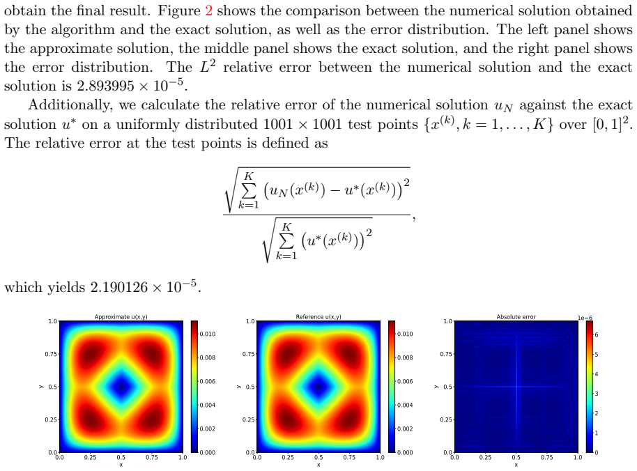
On its own terms, the paper's central discovery is that neural-network subspace approximation can solve second-order elliptic boundary value problems with singular solutions and discontinuous coefficients to high accuracy, provided the integrals in the loss are evaluated by quadrature rules matched to the integrand's singularities or the interface. The analysis decomposes the final error into three terms: the approximation error $\inf_{v\in V_{NN}}\|u-v\|_a$, the integration error $\varepsilon_{int}$, and the optimization error $\varepsilon_{opt}$, and concludes that integration error controls the accuracy when Monte-Carlo or sampling methods are used. In the singular example, Gauss-Jacobi quadrature for the $(x_i-\tfrac12)^{-2/3}$ factors yields a test-point relative error of 2.19e-5, whereas uniform Gauss-Legendre quadrature with 4000 points per dimension yields 4.6e-2. For interface problems, the a posteriori error-estimator loss with composite Gauss-Lobatto integration gives test-point errors of order 1e-8 to 1e-9, including a circular-inclusion problem with non-homogeneous boundary data. The natural conclusion drawn in the paper is that improving the accuracy of the integrations in the loss is the essential step toward high-accuracy neural PDE solvers.
Load-bearing premise
The load-bearing premise is that for each test problem a quadrature rule can be chosen so that the integration error in the loss is negligible for the neural-network integrands; if no such rule is available or the rule does not match the singularity or interface, the high accuracy claimed by the paper collapses.
Editorial extensions
If this is right
- Replacing Monte-Carlo loss evaluation with matched quadrature should improve the accuracy of existing neural PDE methods even when their architecture is unchanged.
- The a posteriori error-estimator loss can act as a built-in error indicator, so the subspace can be refined adaptively without a separate mesh or an external error estimator.
- On the singular benchmark, the machine-learned subspace reaches a test-point relative error around 2e-5, whereas the adaptive linear and quadratic finite element results reported in the paper sit near 2.3e-3 in relative L2 error.
- Interface problems with coefficient contrasts up to 4000 and high-frequency solution components are solved to test-point errors of order 1e-6 to 1e-9, indicating that the adaptively updated subspace can handle low global smoothness.
Reading between the lines
- A natural next test is an interface problem whose geometry is not aligned with tensor-product quadrature, such as an ellipse or a moving front; the method would need an adaptive quadrature construction to keep the integration error negligible.
- Because the a posteriori loss also measures the dual error, it could be repurposed as a stopping criterion or as an indicator for choosing the subspace dimension $p$ rather than fixing it.
- The quadrature-first principle suggests that extending the method to time-dependent or nonlinear PDEs will require quadrature rules matched to the evolving solution's singularities rather than simply larger networks.
Editorial analysis
A structured set of objections, weighed in public.
Referee Report
Summary. The paper proposes an adaptive neural network subspace method for second-order elliptic PDEs. A neural-network-generated basis spans a finite-dimensional subspace, a Galerkin/Ritz solve determines the coefficients, and training updates the network parameters. The authors give an error decomposition into approximation error, numerical integration error, and optimization error, and they argue that high-accuracy quadrature, rather than network expressivity alone, is the key to accurate PDE solutions. They use either a Ritz loss or an a posteriori error-estimator loss derived from a complementarity identity, and they demonstrate the method on a singular Laplace problem and on elliptic interface problems with discontinuous coefficients. Reported test-point relative errors are around 2e-5 for the singular problem and 1e-8 to 1e-9 for straight-interface problems, with a curved-interface example reaching about 5.6e-7. A negative control with uniform Gauss-Legendre quadrature degrades the singular-problem error to 4.6e-2, supporting the paper's emphasis on integration accuracy.
Significance. If the claims are accepted, the paper makes a useful and partially falsifiable point: for low-dimensional elliptic problems, the accuracy ceiling of neural-network methods can be set by the quadrature used to evaluate the loss, not by network capacity. The numerical evidence is strong within the tested problem classes, and the explicit negative control (4000 uniform Gauss-Legendre points per dimension versus tailored Gauss-Jacobi quadrature) is a valuable experiment. The complementarity-based a posteriori estimator (Lemma 3.2) gives an exact identity that clearly explains why the residual-based loss is a sensible objective. The main limitation is that the reported high accuracy relies on quadrature rules constructed from exact knowledge of the singularity location/exponent and of the interface geometry; the paper does not yet provide an automatic mechanism for the general case, so the broad high-accuracy claim is conditional on this prior knowledge.
major comments (3)
- [Section 3, quadrature for loss (3.23)] The singular-problem experiment uses (α,β)-Gauss-Jacobi quadrature with α,β=-2/3 after splitting the domain at x1=1/2 and x2=1/2, i.e., the exact location and exponent of the singularity are encoded in the quadrature rule. The paper gives no procedure for constructing such quadrature when the singularity is unknown in advance, so ε_int in inequality (2.15) is uncontrolled in the general case. The negative control in Section 3 (4000 uniform Gauss-Legendre points per dimension giving 4.601047e-2 versus 2.190126e-5 with Gauss-Jacobi quadrature) confirms that the reported high accuracy is a property of the tailored quadrature rather than of the NN subspace or the loss alone. Please add an automatic quadrature-error control strategy or explicitly state that the high-accuracy claim is restricted to problems whose singularity location and exponent are known and used in the quadrature.
- [Section 2, Eqs. (2.13)-(2.15)] The central error decomposition (2.15) is introduced through inequality (2.13), but ε_int is never defined, and the relation between the quadrature error in the loss functional and the energy-norm difference ∥u^(1)_NN - u^(2)_NN∥_a is not proved. As written, (2.13) is a heuristic statement ('ε_int × some norm of u^(1)_NN'), so the conclusion that integration error always controls machine learning accuracy is not established by the analysis. A rigorous version should specify the quadrature error in a suitable dual norm and the stability constant of the Ritz problem; the numerical section could then be connected to this estimate quantitatively.
- [Section 4.3, loss (4.26) and quadrature] The interface experiments are also built on problem-specific quadrature: composite Gauss-Lobatto rules aligned with the straight interfaces x1=2/3 and x1=2/9, and polar-coordinate quadrature for the circular interface in (4.22). For a curved interface that is not aligned with the quadrature grid and is not given by a simple parametrization, the loss (4.26) cannot be evaluated accurately by the described schemes, so the interface high-accuracy claim is conditional on the interface geometry being known and quadrature-compatible. Please state this limitation and, if the general claim is retained, provide a strategy for automatic interface quadrature (e.g., interface-fitted quadrature or local refinement).
minor comments (6)
- [Throughout] Algorithm 2 heading and Step 2 contain typos ('methd', 'wiht'); Section 3 contains 'It ie easy'; Section 4.1 contains 'adpative' and uses 'un' instead of u_N in the proof of Theorem 4.1; please correct all typographical errors.
- [Section 2, Eqs. (2.11)-(2.12)] The step from (2.11) to (2.12) is the parallelogram law (polarization identity), not the binomial theorem; please rephrase.
- [Section 4, Theorem 4.1 and loss (4.14)] Theorem 4.1 involves the constants λmin and λ1,Γ, but the loss (4.14) drops the multiplicative factor (1+1/λmin+1/λ1,Γ). Since the factor is independent of u_N, the loss remains a valid objective, but the relation between L(u_N) and ∥u-u_N∥_a should be stated as an equivalence with a constant rather than as an equality.
- [Abstract and Section 3] The abstract mentions the hypercircle technique, but Section 3 derives the estimator via Green's formula and the complementarity identity (3.14); the connection to the hypercircle/complementarity method of [28] should be made explicit in the text.
- [Table 6] Table 6 reports etest = 8.96e-01 for standard PINN and 5.20e-04 for nDS-PINN without specifying the network sizes, training schedules, or quadrature used for those baselines; please indicate whether these numbers are taken verbatim from [37] and cite the corresponding settings.
- [Section 3, Eq. (3.21)] The notation in the definition of f and the exact solution (3.21) uses x for the point and later x1, x2 for components; please make the notation uniform.
Circularity Check
No significant circularity: the error decomposition, loss functions, and accuracy claims are independently grounded; self-citations are background only.
full rationale
The paper's derivation chain is self-contained for its central claims. The main error estimate (2.15) separates the total error into a best-approximation error, a quadrature error, and an optimization error; none of these terms is fitted to the reported test errors, and the proof of Theorem 2.1 is given directly. The a posteriori error estimator in Theorem 3.1 is attributed to the external reference [28] and is also proved in the paper; the loss functions (3.12), (3.19), (4.14), and (4.26) are derived from standard residual and hypercircle identities rather than from the numerical solutions being predicted. The numerical experiments use manufactured exact solutions and measure errors against those independent solutions, so the reported accuracies are not outputs of a fitted parameter. The authors do cite their own prior TNN papers [30,31,32,33], but those citations are used to motivate high-accuracy integration for tensor neural networks and are not load-bearing for the low-dimensional singular and interface results; indeed, the paper also tests a two-dimensional FNN subspace and obtains comparable accuracy. The hand-tailored quadrature for the singular example uses the known form of the right-hand side f, which is part of the problem data, and the interface quadrature is aligned with the prescribed interface geometry; this is a scope condition, not a circular reduction. The negative control with uniform Gauss-Legendre quadrature shows degraded accuracy and supports, rather than disguises, the claim that integration accuracy controls the method. No uniqueness theorem is imported from the authors' prior work, and no known empirical pattern is merely renamed. Therefore no specific circular step can be exhibited.
Assumptions & free parameters
free parameters (3)
- Rank p of the neural network subspace =
p = 100
- Quadrature point counts =
200 Gauss-Jacobi points per dimension; 100 subintervals x 8 or 16 Gauss-Lobatto points; 160 theta points for polar…
- Optimizer schedules =
Adam lr=0.001-0.01 for 5,000-50,000 steps; LBFGS lr=0.1-1 for 100-10,000 steps
assumptions (8)
- standard math Lax-Milgram and Ritz equivalence for the symmetric coercive elliptic problem (2.1)-(2.2) produce a unique minimizer satisfying the Galerkin orthogonality (2.8).
- standard math The Poincare inequality holds on H^1_0(Omega), so the first eigenvalue lambda_1 > 0 in (3.5)-(3.6) gives the coercivity ratio ||v||_a / ||v||_0 >= sqrt(lambda_min).
- standard math The hypercircle/complementarity identity (Lemma 3.2, after Vejchodsky [28]) is valid; it equates the squared error sum to eta^2(psi,y).
- standard math The piecewise integration-by-parts formula (4.5) holds for p in H(div,Omega1) cap H(div,Omega2) and v in H^1_0(Omega), including the interface jump term.
- standard math The Steklov eigenvalue problem (4.6)-(4.7) has positive eigenvalues and the trace inequality (4.8) holds.
- domain assumption At each training step, the p neural-network output functions phi_j(.;theta) are linearly independent, so the assembled stiffness matrix A^(ell) is nonsingular and the Galerkin system A^(ell)c = B^(ell) has a unique solution.
- domain assumption The trial functions built by multiplying NN outputs by boundary/interface factors (e.g., (3.22), (4.12), and the sums in Section 4) lie in H^1_0(Omega) and have the differentiability needed to evaluate the residuals in the loss functions (3.12), (3.19), (4.14), and (4.26).
- domain assumption The chosen quadrature rules (Gauss-Jacobi with singular weights, composite Gauss-Lobatto) achieve negligible integration error when applied to the neural-network integrands involved in the loss functions.
Cite this review
Pith. "Pith review of Adaptive Neural Network Subspace Method for Solving Partial Differential Equations with High Accuracy." pith.science (2026). https://pith.science/paper/2UT3VDPQ
@misc{pith2026241202586,
  author       = {Pith},
  title        = {Pith review of: Adaptive Neural Network Subspace Method for Solving Partial Differential Equations with High Accuracy},
  year         = {2026},
  howpublished = {\url{https://pith.science/paper/2UT3VDPQ}},
  note         = {Machine review of arXiv:2412.02586}
}
read the original abstract
Based on neural network and adaptive subspace approximation method, we propose a new machine learning method for solving partial differential equations. The neural network is adopted to build the basis of the finite dimensional subspace. Then the discrete solution is obtained by using the subspace approximation. Especially, based on the subspace approximation, a posteriori error estimator can be derivated by the hypercircle technique. This a posteriori error estimator can act as the loss function for adaptively refining the parameters of neural network.
Figures


Figures from the paper (11 more)


Forward citations
Cited by 2 Pith papers
-
Adaptive feature capture method for solving partial differential equations with near singular solutions
An adaptive random feature method that repositions feature hyperplanes and collocation points according to the gradient of the current approximation resolves near-singular PDEs to high accuracy.
-
Domain Decomposition Subspace Neural Network Method for Solving Linear and Nonlinear Partial Differential Equations
A domain-decomposition subspace neural network method solves linear and nonlinear PDEs with errors down to 1e-13 and lower training cost than PINN, DGM, DRM, and LocELM on 1D/2D benchmarks.
Reference graph
Works this paper leans on
-
[21]
P. Liu, Z. Xu and Z. Sheng, Subspace method based on neural networks for solving the partial differential equation in weak form, arXiv:2405.08513, 2024
arXiv 2024
-
[1]
F. Cao, X. Guo, F. Gao and D. Yuan, Deep learning nonhomogeneous elliptic interface problems by soft constraint physics-informed neural networks, Mathematics 11 (8) (2023), http://dx.doi.org/10.3390/math11081843
-
[2]
J. Chen, X. Chi, W. E and Z. Yang, Bridging traditional and ma chine learning-based algorithms for solving PDEs: the random feature method, J. Mach. Learn., 1 (2022), 268– 298
work page 2022
-
[3]
Z. Chen and Y. Liu, An arbitrarily high order unfitted finite element method for elliptic interface problems with automatic mesh generation, J. Comput. Phys., 491 (2023), 112384
work page 2023
-
[4]
Z. Chen and Y. Liu, An arbitrarily high order unfitted finite element method for elliptic interface problems with automatic mesh generation, Part II. Piecewise-smooth interfaces, Applied Numerical Mathematics, 206 (2024), 247–268. 31
work page 2024
-
[5]
Z. Chen and J. Zou, Finite element methods and their convergence for elliptic and parabolic interface problems, Numer. Math., 79 (1998), 175–202
work page 1998
-
[7]
S. Dong, Z. Li, Local extreme learning machines and domain decomposition for solving linear and nonlinear partial differential equations, Comput. Methods Appl. Mech. Engrg., 387 (2021), 114129
work page 2021
-
[8]
S. Dong, Z. Li, A modified batch intrinsic plascity method for pretraining the random coefficients of extreme learning machines, J. Comput. Phys., 445 (2021), 110585
work page 2021
Show all 38 references
-
[9]
W. E and B. Yu, The deep Ritz method: a deep-learning based numerical algorithm for solving variational problems, Commun. Math. Stat., 6 (2018), 1–12
2018
-
[10]
J. Han, L. Zhang and W. E, Solving many-electron Schr¨ odinger equation u sing deep neural networks. J. Comput. Phys., 399 (2019), 108929
2019
-
[11]
C. He, X. Hu and L. Mu, A mesh-free method using piecewise deep neural network for elliptic interface problems, J. Comput. Appl. Math., 412 (2022), 114358, http://dx.doi. org/10.1016/j.cam.2022.114358
2022
-
[12]
Huang and R
W. Huang and R. D. Russell, Adaptive Moving Mesh Methods, Applied Mathematical Sciences, vol 174. Springer, New York, NY, 2010
2010
-
[13]
Z. Hu, K. Shukla, G. E. Karniadakis and K. Kawaguchi, Tackling the curse of dimension- ality with physics-informed neural networks, arXiv:2307.12306v5, 2024
2024 arXiv
-
[14]
G. Hu, Z. Qiao, and T. Tang, Moving finite element simulations for reaction–diffusion systems, Adv. Appl. Math. Mech., 4(03) (2012), 365–381
2012
-
[15]
Huang, Q
G. Huang, Q. Zhu, C. Siew, Extreme learning machine: theory and applications, Neuro- computing, 70 (2006), 489–501
2006
-
[16]
T. Kao, J. Zhao and L. Zhang, pETNNs: partial evolutionary tensor neural networks for solving time-dependent partial differential equations, arXiv:2403.06084v1, 2024
2024
-
[17]
D. P. Kingma and J. Ba, Adam: A method for stochastic optimization, arXiv:1412.6980, 2014; Published as a conference paper at ICLR 2015
2014 arXiv
-
[18]
J. Li, J. M. Melenk, B. Wohlmuth and J. Zou, Optimal a priori estimates for higher order finite elements for elliptic interface problems, Applied Numerical Mathematics, 60 (2010), 19–37
2010
-
[19]
R. Li, T. Tang and P. Zhang, Moving mesh methods in multiple dimensions based on harmonic maps, J. Comput. Phys., 170(2) (2001), 562–588
2001
-
[20]
Y. Li, F. Wang, Local randomized neural networks methods for interface problems, arXiv:2308.03087, 2023
2023 arXiv
-
[22]
W. F. Mitchell, A collection of 2D elliptic problems for testing adaptive grid refinement algorithms, Applied mathematics and computation, 220 (2013), 350–364. 32
2013
-
[23]
Raissi, P
M. Raissi, P. Perdikaris and G. E. Karniadakis, Physics informed deep learning (part I): Data-driven solutions of nonlinear partial differential equations, arXiv:1711.10561, 2017
2017 arXiv
-
[24]
Shang, F
Y. Shang, F. Wang and J. Sun, Randomized neural network with Petrov-Galerkin methods for solving linear and nonlinear partial differential equations, Communications in Nonlinear Science and Numerical Simulation, 127 (2023), 107518
2023
-
[25]
J. Shen, T. Tang and L. Wang, Spectral methods: algorithms, analysis and applications: volume 41, Springer Science & Business Media, 2011
2011
-
[26]
Sirignano and K
J. Sirignano and K. Spiliopoulos, DGM: A deep learning algorithm for solving partial differential equations, J. Comput. Phys., 375 (2018), 1339–1364
2018
-
[27]
J. Sun, S. Dong and F. Wang, Local randomized neural networks with discontinuous Galerkin methods for partial differential equations, J. Comput. Appl. Math., 445 (2024), 115830
2024
-
[28]
Vejchodsk` y, Complementarity based a posteriori error estimates and their properties, Math
T. Vejchodsk` y, Complementarity based a posteriori error estimates and their properties, Math. Comput. Simulat., 82(10) (2012), 2033–2046
2012
-
[29]
T. Wang, Z. Hu, K. Kawaguchi, Z. Zhang and G. E. Karniadakis, Tensor neural networks for high-dimensional Fokker-Planck equations, arXiv:2404.05615v1, 2024
2024 arXiv
-
[30]
Y. Wang, P. Jin and H. Xie, Tensor neural network and its numerical integration, arXiv:2207.02754, 2022
2022 arXiv
-
[31]
Y. Wang, Y. Liao and H. Xie, Solving Schr¨ odinger equation using tensor neural network, arXiv:2209.12572, 2022
2022 arXiv
-
[32]
Y. Wang, Z. Lin, Y. Liao, H. Liu and H. Xie, Solving high dimensional partial differential equations using tensor neural network and a posteriori error estimators, arXiv:2311.02732, 2023
2023 arXiv
-
[33]
Wang and H
Y. Wang and H. Xie, Computing multi-eigenpairs of high-dimensional eigenvalue problems using tensor neural networks, J. Comput. Phys., 506 (2024), 112928 (arXiv:2305.12656, 2023)
2024 arXiv
-
[34]
Wu and B
S. Wu and B. Lu, INN: Interfaced neural networks as an accessible meshless approach for solving interface PDE problems, J. Comput. Phys., 470 (2022), 111588, http://dx.doi. org/10.1016/j.jcp.2022.111588
2022
-
[35]
Y. Xie, H. Chi, Y. Wang and Y. Ma, Physics-specialized neural network with hard con- straints for solving multi-material diffusion problems, Computer Methods in Applied Me- chanics and Engineering, 430 (2024), 117223
2024
-
[36]
Xu and Z
Z. Xu and Z. Sheng, Subspace method based on neural networks for solving the partial differential equation, arXiv:2404.08223, 2024
2024 arXiv
-
[37]
Y. Yao, J. Guo and T. Gu, A deep learning method for multi-material diffusion problems based on physics-informed neural networks, Computer Methods in Applied Mechanics and Engineering, 417 (2023), 116395
2023
-
[38]
Y. Zang, G. Bao, X. Ye and H. Zhou, Weak adversarial networks for high-dimensional partial differential equations, J. Comput. Phys., 411 (2020), 109409. 33
2020
-
[39]
Zhou and Z
H. Zhou and Z. Sheng, Improved randomized neural network methods with boundary processing for solving elliptic equations, arXiv:2407.18457, 2024. 34
2024 arXiv
Reviewed August 11, 2026 · model on record in the stance chip above.
Discussion (0). Continue with ORCID to comment.