Provable Uncertainty Decomposition via Higher-Order Calibration

Aravind Gollakota; Charlotte Peale; Gustaf Ahdritz; Parikshit Gopalan; Udi Wieder

REVIEW 1 major objections 5 minor 13 references

Provable Uncertainty Decomposition via Higher-Order Calibration

T0 review · 1 major / 5 minor · reviewed 2026-08-11 · deepseek-v4-flash

Challenge this review Re-run · record.json Download PDF Read on arXiv ↗ Review JSON

Pith's one-line read Aleatoric uncertainty estimates get a provable real-world meaning

desk verdict A clean and genuinely useful formalization of higher-order calibration; the main framework holds up, but the moment-based prediction-set section has a concrete sign error that needs fixing. read the letter →

arxiv 2412.18808 v1 pith:OXO3NQMV submitted 2024-12-25 cs.LG cs.CVstat.ML

Gustaf Ahdritz , Aravind Gollakota , Parikshit Gopalan , Charlotte Peale , Udi Wieder This is my paper · ORCID

classification cs.LGcs.CVstat.ML

keywords higher-ordercalibrationkth-orderk-snapshotsaleatoricuncertaintyepistemicdecompositionmixturelearning

verification ladder T0 review T1 audit T2 compute T3 formal

The pith

A machine-rendered reading of the paper's core claim, the machinery that carries it, and where it could break.

The reading

This paper introduces higher-order calibration, a calibration notion for predictors that output mixtures of label distributions, and proves that under it the estimated aleatoric uncertainty—the part of predictive uncertainty caused by inherent randomness in the data—equals the average true aleatoric uncertainty over all points with the same prediction. Because the true mixture is unobservable, the paper defines kth-order calibration using k-snapshots, i.e., k independent labels per instance, and shows it can be both measured and achieved without any assumptions on the data distribution. It proves that kth-order calibration converges to higher-order calibration at a $1/\sqrt{k}$ rate, and that small k already suffices for common entropy functions such as Brier. This matters because it gives practitioners a distribution-free way to tell whether a model's uncertainty reflects genuine data ambiguity or model ignorance.

What carries the argument

The load-bearing object is the $k$th-order projection $\operatorname{proj}_k(\pi)$, which turns a mixture of label distributions into the distribution over normalized histograms of $k$ iid label draws; this makes higher-order calibration checkable from observable k-snapshot data. Combined with the Wasserstein-1 metric on mixtures, it yields the convergence bound (kth-order calibrated implies $(\epsilon + |Y|/(2\sqrt{k}))$-higher-order calibrated), exact recovery of the first $k$ moments, and a post-hoc mixture-learning procedure. The mutual information decomposition with a concave generalized entropy $G$ then converts a predicted mixture into predictive, aleatoric, and epistemic components.

What would settle it

Using a dataset where each point has many independent annotations so that $f^*(x)$ is known up to sampling noise, train a kth-order calibrated predictor, bin the points by prediction, and compare the predicted average entropy in each bin with the true average entropy of the normalized label histograms; a systematic gap beyond the stated $\epsilon$ would show the calibration guarantee does not deliver its promised real-world semantics.

Watch

Extended reading notes

Core claim

The central claim is that a higher-order calibrated predictor—one whose prediction at every point equals the Bayes mixture over its level set—automatically gives a correct uncertainty decomposition: the average entropy of the predicted mixture components equals the average true aleatoric uncertainty over the level set, and the epistemic term equals the average divergence of the true label distributions from their centroid. The paper states this as the first guarantee of its kind that makes no assumptions on the real-world distribution. It also extends the guarantee to kth-order calibration, proving recovery of the first k moments of the Bayes mixture and giving entropy estimates for Brier and Shannon entropies from snapshot-calibrated predictors.

Load-bearing premise

The k labels in a k-snapshot must be independent draws from the same true conditional distribution $f^*(x)$ at that instance; if repeated labels are biased or correlated, the observed snapshot distribution is not the kth-order projection of the Bayes mixture and the guarantees no longer apply.

Editorial extensions

If this is right

A higher-order calibrated model's aleatoric uncertainty estimate is correct in aggregate over every equivalence class, so model diagnostics can separate data ambiguity from model ignorance without distributional assumptions.
Any existing higher-order predictor, such as a Bayesian or ensemble model, can be evaluated with a concrete kth-order calibration metric instead of relying on the model class being well-specified.
kth-order calibration is achievable by reducing to first-order calibration over the extended label space of k-snapshots, and a post-hoc variant needs only a calibration set of snapshots.
Small snapshot sizes give usable guarantees: second-order calibration suffices for Brier-entropy aleatoric estimates, and kth-order calibration yields moment-based prediction sets with coverage at least $1-\alpha$.
Larger $k$ improves the approximation of full higher-order calibration at a quantifiable $1/\sqrt{k}$ rate, so users can trade labeling budget against guaranteed accuracy.

Reading between the lines

Editorial extensions of the paper, not claims the author makes directly.

An implication left implicit is that the same post-hoc calibration routine can audit the epistemic uncertainty of deep ensembles or Bayesian neural networks: build the level-set partition of the model, collect k-snapshots per bin, and measure the Wasserstein distance to the empirical snapshot distribution.
A natural extension is a labeling-budget rule: since the approximation error shrinks as $1/\sqrt{k}$, the bounds suggest that beyond a few dozen labels per point, additional labels buy little extra guarantee.
The independence assumption on the k labels is the likely failure point in practice; modeling correlated annotators as a perturbed snapshot distribution and quantifying the resulting degradation of the decomposition guarantees would be a direct follow-up the paper does not analyze.

Share X Bluesky LinkedIn Reddit HN

Signed reviews

No signed human review yet.

Editorial analysis

A structured set of objections, weighed in public.

Desk editor's note, referee report, and a circularity audit.

Desk Editor's Note

read the letter

First thing to know: this is a solid paper. It takes JTDM24's k=2 second-order calibration and turns it into a proper hierarchy: kth-order calibration, limiting higher-order calibration, convergence at 1/√k, moment recovery, entropy estimation, and prediction sets. The central semantics are exactly what the definition says—Theorem 1.2 is essentially immediate from higher-order calibration—but making that definition explicit is a real contribution, and the surrounding machinery is not just definition-chasing. The moment recovery lemma (3.5) and the Wasserstein-based prediction set theorem (5.3) are clean, and the entropy estimation results via polynomial approximation are genuinely useful. The experiments on CIFAR-10H and FER+ are suggestive, and the paper is honest about the k-snapshot requirement.

Now the soft spots. Section 5.1 has a real error. Corollary 5.4 expands E[(p − m1)^k] as if it were Σ C(k,i) E[p^i] m1^{k−i}. The alternating signs from (−m1)^{k−i} are missing. The estimator c_k they define is not a central-moment estimate; for a degenerate mixture at p=0.5, k=2, exact moments give c_2 = 1 while the central moment is 0. So Theorem 5.5's moment-based prediction sets are not established. This is localized—it does not touch Theorem 5.3 or the main decomposition results—but it is a genuine flaw and needs to be fixed, or that subsection removed.

A smaller issue: Theorem 4.3 is stated generally, but the detailed entropy-estimation proof and sample complexity are worked out only for the binary case. It should say so in the statement. And there is a mild overclaim in the abstract: the 'first formal guarantee with no assumptions' is true by the definition, and it still assumes k-snapshots are iid draws from f*(x). The authors acknowledge this, but the abstract could be more careful.

No code is shipped, so the experiments are not independently reproducible as-is. That is a minor point given the theory carries the paper.

Who is this for? Anyone working on uncertainty quantification for Bayesian or ensemble models, and theory-minded ML folks who want a distribution-free semantics for aleatoric/epistemic splitting. It deserves a serious referee. I would accept it with a request for major revision that fixes the sign error and clarifies the binary-only proofs.

Referee Report

1 major / 5 minor

Summary. The paper introduces a theory of higher-order calibration for predictors f: X → ΔΔY, where the predicted object is a mixture over label distributions. A predictor is higher-order calibrated if, on each of its level sets [x], the predicted mixture equals the Bayes mixture f*([x]) formed by the true conditional distributions f*(x) over x ∼ [x]. The paper then defines kth-order calibration, a relaxation based on k-snapshots, i.e., k independent labels drawn from f*(x), and shows that kth-order calibration is tractable to verify and achieve, converges to higher-order calibration at rate |Y|/(2√k), and recovers the first k moments of the Bayes mixture. These tools are used to give semantics for the standard aleatoric/epistemic uncertainty decomposition (Theorem 1.2), to estimate common entropy functions (Theorem 4.3), and to construct higher-order prediction sets (Section 5). Experiments on CIFAR-10H and FER+ demonstrate that snapshot-based calibration improves estimates of aleatoric uncertainty.

Significance. If the results hold, this is a substantial contribution to uncertainty quantification: it provides a distribution-free, frequentist semantics for aleatoric/epistemic decomposition and a practical relaxation based on multiple labels per instance. The paper's strengths are the explicit chain from k-snapshot data to distributional guarantees: the Wasserstein projection bound (Lemma D.3), moment-recovery estimators (Lemma D.8 and Theorem 3.5), and finite-sample calibration procedures (Theorem 3.6) are clean and appear correct. The experiments support the practical value of the approach. One caveat is that Theorem 1.2 is an immediate substitution into Definition 1.1; the substantive content lies in the kth-order relaxation, moment recovery, and entropy-estimation results. The moment-based prediction-set subsection contains an algebraic error that must be repaired, although the main uncertainty-decomposition claims are unaffected.

major comments (1)

[§5.1, Corollary 5.4] The binomial expansion of E[(p−m1)^k] is incorrect: it omits the alternating signs and should read Σ_{i=0}^k C(k,i) E[p^i] (−m1)^{k−i}. As defined, c_k is not a central-moment estimate. For example, with k=2 and a mixture degenerate at p=0.5, the exact moments are m1=0.5, m2=0.25; the paper's c_2 equals 1.0, while E[(p−m1)^2]=0, contradicting the claimed error bound of 0 when ϵ=0. Consequently, the Markov step in Theorem 5.5 does not follow as written, so the moment-based higher-order prediction-set guarantee is not established by the submitted proof. The result appears repairable, because for p,m1≥0 one has |p−m1|^k ≤ (p+m1)^k, so c_k is naturally an estimate of E[(p+m1)^k], an upper bound on the desired central moment; however, the authors must restate Corollary 5.4 and prove Theorem 5.5 using this inequality rather than the false central-moment identity.

minor comments (5)

[§5.1, Corollary 5.4] The vector of moment estimates is written as (m1,...,mk) ∈ R^n; this should be R^k.
[§4, Theorem 4.3] The Shannon-entropy bullet states 'k ≥ Θ((1/ϵ)ln 4)', which reads as a logarithmic dependence on 1/ϵ. The formal statement in Corollary E.9 has k ≥ (1/4)(2C1/ϵ)^{ln4}, which is a polynomial dependence with exponent ln4. Please align the informal and formal statements.
[§6] The CIFAR-10H experiments construct f*(x) as the uniform distribution over all available annotations and then sample k-snapshots from this histogram. This implicitly assumes that human annotators produce iid draws from f*(x); a brief discussion of how annotator dependence or systematic bias would affect the empirical evaluation would strengthen the paper, even though the theoretical model explicitly assumes independence.
[§1.2, Definition 3.2] The phrase 'empirical distribution of k-snapshots' in the informal discussion is easily confused with a finite-sample empirical measure; consider using 'the distribution of a randomly drawn k-snapshot' to distinguish it from the empirical estimate in Theorem 3.6.
[Appendix E.2, Corollary E.9] The proof uses both exp(C4(1/ϵ)^{ln4}) and exp(C4(1/ϵ)ln4) in the same paragraph; the notation should be made unambiguous, since the two expressions are very different in magnitude.

Circularity Check

1 steps flagged · score 4.0 of 10

Partial circularity: the central aleatoric-uncertainty guarantee is an unpacking of the definition of higher-order calibration, though the kth-order relaxation and prediction-set results are independent.

self definitional [Definition 1.1 and Lemma 4.2 (Theorem 1.2)]
"We say f is higher-order calibrated if for every x, f (x) = f ∗([x]). ... Since f (x) = f ∗([x]) as a mixture, AU_G(f : x) = E_{p∼f (x)}[G(p)] = E_{p∗∼f ∗([x])}[G(p∗)] = E_{x∼[x]}[G(f ∗(x))] = E_{x∼[x]}[AU∗_G(x)]."

The theorem's conclusion is obtained by substituting the defining equality f(x)=f*([x]) into Definition 4.1 of AU_G and into the definition of f*([x]) as the Bayes mixture over [x]. Since AU*_G(x)=G(f*(x)) by definition, Lemma 4.2 is the same statement as Definition 1.1 with G applied to both sides: E_{p~f(x)}G(p) = E_{x~[x]}G(f*(x)). Thus the 'real-world' aleatoric guarantee is not derived from independent evidence; it is the calibration definition rewritten in entropy notation. The semantic content is imposed by the definition rather than proven.

full rationale

The flagged step is a genuine self-definitional reduction: Theorem 1.2's aleatoric bullet adds no assumption beyond Definition 1.1; it just applies G to both sides of the defining equality. However, the paper's remaining contributions are not circular. The kth-order projection formalism (Definitions 3.2-3.3), the convergence rate (Theorem 3.4 via Lemma D.3), moment recovery with the explicit estimator M_{k,m} (Theorem 3.5/Lemma D.8), post-hoc calibration sample bounds (Theorem 3.6), entropy-estimation reductions (Theorems 4.3, E.4, E.7), the MGF-based equivalence (Theorem 4.4), and the Wasserstein prediction-set transfer (Theorem 5.3) are proved from stated assumptions with independent arguments. Self-citations to [BGHN23, GOR+24, GHR24] are related-work pointers and are not load-bearing. Section 7's stated limitation (k>1 requires multiple independent labels per instance) is an applicability constraint, not a circular step. The score of 4 reflects one central definitional reduction while acknowledging substantial independent technical content; it is not a claim that the whole derivation is a fit renamed as prediction.

Assumptions & free parameters 0 free parameters · 4 assumptions · 0 invented entities

The central claim rests on the definition of higher-order calibration and on the data model where k labels per instance are iid draws from f*(x). The entropy-estimation theorems use standard approximation theory and proper-loss results. There are no fitted constants or invented physical entities.

assumptions (4)

domain assumption For each instance x, the k labels in a k-snapshot are independent draws from the same conditional distribution f*(x).
This is the data model introduced in Section 1.2 and Definition 3.2. If annotators are not independent or have different biases, the empirical snapshot distribution does not equal proj_k f*([x]) and the kth-order calibration guarantees fail.
standard math Every concave generalized entropy function G corresponds to a proper loss (Gneiting-Raftery 2007).
Used in Section 4 and Appendix C to justify the generalized entropy framework and the equivalence in Theorem 4.4.
standard math Jackson's theorem on polynomial approximation of uniformly continuous functions.
Used in Theorem 4.3 and Corollary E.9 to approximate Shannon entropy by low-degree polynomials on the binary simplex.
standard math Moment generating functions uniquely determine distributions on the bounded simplex.
Used in the proof of Theorem 4.4 (Appendix E.1) to show that matching all concave-function expectations forces the predicted mixture to equal the Bayes mixture.

how reviews work

0 comments

Cite this review

Pith. "Pith review of Provable Uncertainty Decomposition via Higher-Order Calibration." pith.science (2026). https://pith.science/paper/OXO3NQMV

@misc{pith2026241218808,
  author       = {Pith},
  title        = {Pith review of: Provable Uncertainty Decomposition via Higher-Order Calibration},
  year         = {2026},
  howpublished = {\url{https://pith.science/paper/OXO3NQMV}},
  note         = {Machine review of arXiv:2412.18808}
}

abstract

We give a principled method for decomposing the predictive uncertainty of a model into aleatoric and epistemic components with explicit semantics relating them to the real-world data distribution. While many works in the literature have proposed such decompositions, they lack the type of formal guarantees we provide. Our method is based on the new notion of higher-order calibration, which generalizes ordinary calibration to the setting of higher-order predictors that predict mixtures over label distributions at every point. We show how to measure as well as achieve higher-order calibration using access to $k$-snapshots, namely examples where each point has $k$ independent conditional labels. Under higher-order calibration, the estimated aleatoric uncertainty at a point is guaranteed to match the real-world aleatoric uncertainty averaged over all points where the prediction is made. To our knowledge, this is the first formal guarantee of this type that places no assumptions whatsoever on the real-world data distribution. Importantly, higher-order calibration is also applicable to existing higher-order predictors such as Bayesian and ensemble models and provides a natural evaluation metric for such models. We demonstrate through experiments that our method produces meaningful uncertainty decompositions for image classification.

Figures

Figures reproduced from arXiv: 2412.18808 by the authors.

**Figure 1.** An illustration of higher-order calibration using the X-ray classification example. We depict scenarios 1 and 2 on the top and bottom respectively. On the left, we have instances grouped together into one level set [x] by the predictor. By learning from snapshots drawn from the level set in either case, we are able to predict mixtures that match the true Bayes mixture f ∗ ([x]). notion in the prediction literature i… view at source ↗

**Figure 2.** Calibrating models with k-snapshots yields increasingly accurate estimates of aleatoric uncertainty. Top: Average aleatoric uncertainty estimation error (Eq. (6.1)) of CIFAR-10 models calibrated using snapshots of increasing size. Bottom: For three of the highest-entropy equivalence classes, we depict the distribution of entropies ranging over components of the predicted mixture (gray) and the Bayes mixture (green)… view at source ↗

**Figure 3.** Qualitatively, accurate estimates of aleatoric uncertainty help separate unusual, poorly learned images (mostly epistemic) from genuinely ambiguous ones (mostly aleatoric). Top: CIFAR-10H images with the highest ratio of epistemic uncertainty to aleatoric uncertainty (depicted by colored bars), as estimated by a well-higher-order-calibrated model. Bottom: The most aleatoric images according to the same model. uncert… view at source ↗

Figures from the paper (3 more)

**Figure 4.** Figure 4: Comparison of Shannon and Brier binary entropy functions. Here we use the scaled version of [PITH_FULL_IMAGE:figures/full_fig_p026_4.png]

**Figure 5.** Figure 5: The simple binary regression task from [JTDM24]. (Positive) inputs are drawn from a normal distribution (left), and outputs are determined by a fixed function p(y|x) (right) with low- and high-frequency components, the latter of which our simple predictor (k = 1) fails…

**Figure 6.** Figure 6: Top: Average aleatoric uncertainty estimation error (Eq. (6.1)) of binary regression models calibrated using snapshots of increasing size. Bottom: For three of the highest-entropy equivalence classes, we depict the distribution of entropies ranging over components of t…

Discussion (0). Continue with ORCID to comment.

Reference graph

Works this paper leans on

13 extracted references · 9 canonical work pages

[1]

,yk ∼ p iid

As a k-snapshot distribution, an object in ∆Y k: The k-snapshot projection of a mixture π is the k-tuple distribution arising from drawing a random p ∼ π, and drawing y1, . . . ,yk ∼ p iid

work page
[2]

As a kth-moment tensor, an object in ( Rℓ)⊗k: The kth-moment tensor of a mixture π is exactly the object E[p⊗k], where p ∼ π.10

work page
[3]

does not require cast

As a symmetrized k-snapshot distribution, an object in ∆Y (k): The symmetrized k-snapshot projection of a mixture π is the distribution arising from drawing p ∼ π, then drawing ( y1, . . . ,yk) ∼ p, and considering Unif( y1, . . . ,yk). This is how we originally defined proj kπ (see Definition 3.2). Observe that the pmf of the k-snapshot projection of π i...

work page
[10]

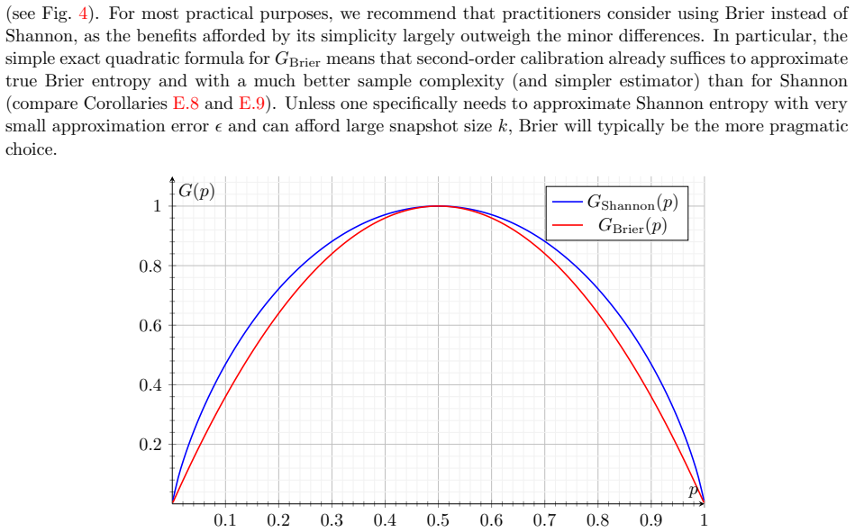
Shannon entropy, GShannon(p) = P y∈Y py log 1 py . The associated loss LShannon(p ∥ p′) = P y∈Y py log 1 p′y is the cross-entropy loss, and the associated divergence DShannon(p ∥ p′) = P y∈Y py log py p′y is precisely the KL divergence. The associated pointwise loss function is the log loss, LShannon(y ∥ p) = log 1 py . In the binary case, GShannon : [0, ...

work page
[11]

supergradient

Brier entropy GBrier(p) = 1 − ∥p∥2 (also known by many other names, including Gini impurity). The associated loss turns out to be LBrier(p ∥ p′) = ∥p − p′∥2 + 1 − ∥p∥2, and the associated divergence DBrier(p ∥ p′) = ∥p − p′∥2 is precisely the squared Euclidean distance. The associated pointwise loss function is (the negation of) the Brier score, LBrier(y ...

work page
[12]

Every Gt ∈ Gis concave

work page
[13]

Naive NN

AU Gt (f : x) and Ex∼[x][AU∗ Gt (x)] are finite for all Gt ∈ G. With these two assumptions, the proof is quickly complete. In particular, if all Gt are concave, then by the main assumption of our theorem, we have AUGt (f : x) = E x∼[x] [AU∗ Gt (x)] for all Gt ∈ G. The equivalences shown in E.1 and E.2 imply that we also have Mp(t) = Mp∗(t) for all t ∈ [−1...

work page
[1981]

Uncertain: Modern topics in uncertainty estimation

E.6 [Rot22] Aaron Roth. Uncertain: Modern topics in uncertainty estimation. Unpublished Lecture Notes, page 2, 2022. B [SAIH23] Kajetan Schweighofer, Lukas Aichberger, Mykyta Ielanskyi, and Sepp Hochreiter. Intro- ducing an improved information-theoretic measure of predictive uncertainty. arXiv preprint arXiv:2311.08309, 2023. 1.3, C, C.3 [SBCH23] Yusuf S...

arXiv 2022

Show all 13 references

[2018]

A survey on uncertainty estimation in deep learning classification systems from a bayesian perspective.ACM Computing Surveys (CSUR), 54(9):1– 35, 2021

1.3 [MPV21] Jos´ e Mena, Oriol Pujol, and Jordi Vitri` a. A survey on uncertainty estimation in deep learning classification systems from a bayesian perspective.ACM Computing Surveys (CSUR), 54(9):1– 35, 2021. 1.3 [Nat64] I.P. Natanson. Constructive Function Theory , volume 1 ...

2021
[2019]

From predictions to decisions: The importance of joint predictive distributions

B [WOQ+21] Zheng Wen, Ian Osband, Chao Qin, Xiuyuan Lu, Morteza Ibrahimi, Vikranth Dwaracherla, Mohammad Asghari, and Benjamin Van Roy. From predictions to decisions: The importance of joint predictive distributions. arXiv preprint arXiv:2107.09224 , 2021. 1.3 [WSH+23] Lisa Wi...

2021 arXiv
[2023]

Distribution calibration for regression

B [SDKF19] Hao Song, Tom Diethe, Meelis Kull, and Peter Flach. Distribution calibration for regression. In International Conference on Machine Learning , pages 5897–5906. PMLR, 2019. B [SFSPN+23] Telmo Silva Filho, Hao Song, Miquel Perello-Nieto, Raul Santos-Rodriguez, Meelis ...

2019 arXiv
[2024]

De- composition of uncertainty in bayesian deep learning for efficient and risk-sensitive learning

1.3 [DHLDVU18] Stefan Depeweg, Jose-Miguel Hernandez-Lobato, Finale Doshi-Velez, and Steffen Udluft. De- composition of uncertainty in bayesian deep learning for efficient and risk-sensitive learning. In International conference on machine learning , pages 1184–1193. PMLR, 201...

2018 arXiv
[2678]

B, B [JMB+24] Mira J¨ urgens, Nis Meinert, Viktor Bengs, Eyke H¨ ullermeier, and Willem Waegeman

PMLR, 2021. B, B [JMB+24] Mira J¨ urgens, Nis Meinert, Viktor Bengs, Eyke H¨ ullermeier, and Willem Waegeman. Is epistemic uncertainty faithfully represented by evidential deep learning methods? arXiv preprint arXiv:2402.09056, 2024. B [JTDM24] Daniel D. Johnson, Daniel Tarlow...

2021 arXiv

Pith tools

Reviewed August 11, 2026 · model on record in the stance chip above.

[1] [1]

,yk ∼ p iid

As a k-snapshot distribution, an object in ∆Y k: The k-snapshot projection of a mixture π is the k-tuple distribution arising from drawing a random p ∼ π, and drawing y1, . . . ,yk ∼ p iid

work page

[2] [2]

As a kth-moment tensor, an object in ( Rℓ)⊗k: The kth-moment tensor of a mixture π is exactly the object E[p⊗k], where p ∼ π.10

work page

[3] [3]

does not require cast

As a symmetrized k-snapshot distribution, an object in ∆Y (k): The symmetrized k-snapshot projection of a mixture π is the distribution arising from drawing p ∼ π, then drawing ( y1, . . . ,yk) ∼ p, and considering Unif( y1, . . . ,yk). This is how we originally defined proj kπ (see Definition 3.2). Observe that the pmf of the k-snapshot projection of π i...

work page

[4] [10]

Shannon entropy, GShannon(p) = P y∈Y py log 1 py . The associated loss LShannon(p ∥ p′) = P y∈Y py log 1 p′y is the cross-entropy loss, and the associated divergence DShannon(p ∥ p′) = P y∈Y py log py p′y is precisely the KL divergence. The associated pointwise loss function is the log loss, LShannon(y ∥ p) = log 1 py . In the binary case, GShannon : [0, ...

work page

[5] [11]

supergradient

Brier entropy GBrier(p) = 1 − ∥p∥2 (also known by many other names, including Gini impurity). The associated loss turns out to be LBrier(p ∥ p′) = ∥p − p′∥2 + 1 − ∥p∥2, and the associated divergence DBrier(p ∥ p′) = ∥p − p′∥2 is precisely the squared Euclidean distance. The associated pointwise loss function is (the negation of) the Brier score, LBrier(y ...

work page

[6] [12]

Every Gt ∈ Gis concave

work page

[7] [13]

Naive NN

AU Gt (f : x) and Ex∼[x][AU∗ Gt (x)] are finite for all Gt ∈ G. With these two assumptions, the proof is quickly complete. In particular, if all Gt are concave, then by the main assumption of our theorem, we have AUGt (f : x) = E x∼[x] [AU∗ Gt (x)] for all Gt ∈ G. The equivalences shown in E.1 and E.2 imply that we also have Mp(t) = Mp∗(t) for all t ∈ [−1...

work page

[8] [1981]

Uncertain: Modern topics in uncertainty estimation

E.6 [Rot22] Aaron Roth. Uncertain: Modern topics in uncertainty estimation. Unpublished Lecture Notes, page 2, 2022. B [SAIH23] Kajetan Schweighofer, Lukas Aichberger, Mykyta Ielanskyi, and Sepp Hochreiter. Intro- ducing an improved information-theoretic measure of predictive uncertainty. arXiv preprint arXiv:2311.08309, 2023. 1.3, C, C.3 [SBCH23] Yusuf S...

arXiv 2022