Regularized dynamical parametric approximation of stiff evolution problems

Christian Lubich; J\"org Nick

REVIEW 2 major objections 4 minor 2 cited by

Regularized dynamical parametric approximation of stiff evolution problems

T0 review · 2 major / 4 minor · reviewed 2026-08-10 · deepseek-v4-flash

Challenge this review Re-run · record.json Download PDF Read on arXiv ↗

Pith's one-line read The paper proves that a regularized parametric implicit Euler method, and its higher-order Runge–Kutta analogues, inherit the stiffness-independent error bound of the underlying integrator up to the size of the regularized residual.

desk verdict First rigorous analysis of regularized parametric implicit integrators for stiff evolution; the conditional error bound is real, but the numerics do not actually enforce its central hypothesis and should be read as illustration, not validation. read the letter →

arxiv 2501.12118 v1 pith:NYBN5GWU submitted 2025-01-21 math.NA cs.LGcs.NA

Christian Lubich , Jörg Nick This is my paper · ORCID

classification math.NAcs.LGcs.NA MSC 65L0465L0665M20

keywords parametrictimeintegrationstiffevolutionequationsimplicitRunge-KuttaGauss-Newtoniterationregularizationneuralnetworkparametrizationdefect-basederrorboundsB-convergence

verification ladder T0 review T1 audit T2 compute T3 formal

The pith

A machine-rendered reading of the paper's core claim, the machinery that carries it, and where it could break.

The reading

The paper addresses the practical problem of evolving a nonlinear parametrized ansatz u(t)=Φ(θ(t))—for example a neural network—along a stiff evolution equation, where the derivative Φ′(θ) can be arbitrarily close to rank-deficient. It proposes regularized parametric versions of implicit Euler and implicit Runge–Kutta integrators, solving each step by a few Gauss–Newton iterations on an ill-conditioned least-squares problem. The central result is that, provided the regularized residuals stay small enough, the parameterized solution satisfies a global error bound of the form O(h+δ) (or O(h^s+δ) for s-stage Radau/Gauß methods) with constants that do not depend on the stiffness. This gives a theoretical foundation for evolutionary neural-network and tensor-network solvers on stiff problems, where explicit parametric integrators suffer from severe step-size restrictions or ill-posedness.

What carries the argument

At the center of the argument is the regularized Gauss–Newton iteration (4.1), which determines each parameter increment $\Delta\theta^k$ by minimizing $$\|(I-hJ_0)\Phi'(\theta_0)\$\Delta$\$\theta$^k/h + r^k\|^2 + \tfrac12\$varepsilon^{2}$\|\$\Delta$\$\theta$^k/h+\$\sigma$^k\|$_Q^{2}$ + \$varepsilon^{2}$\|\$\Delta$\$\theta$^k/h\|$_Q^{2}$,$$ where $r^k$ is the current residual of the implicit-Euler step and $\sigma^k$ the current parameter velocity. The extra regularization terms compensate for the arbitrarily small singular values of $\Phi'(\theta_0)$, and the resulting defect $\delta^k$ controls both the residual and the parameter movement. The proof compares these iterates to the Newton iterates of the non-parametric integrator, giving the recursive bound of Theorem 4.1; for Runge–Kutta methods the same structure is diagonalized through the coefficient matrix, reducing the analysis to independent scalar least-squares problems.

What would settle it

Implement the regularized parametric implicit Euler method on a stiff linear heat equation with smooth initial data and a flexible parametrization, choosing h and ε so the residual bound h($δ^{{K−1}}$+...+$δ^{0}$)≤cε² is satisfied. If for some such choice the observed global error exceeds C1δ+C2η with constants that remain uniform as the diffusion coefficient is increased, the claimed stiffness-independent bound is false.

Watch

Extended reading notes

Core claim

At the heart of the proof is a comparison between the regularized Gauss–Newton iterates actually computed and the Newton iterates of the non-parametric implicit integrator, which are a theoretical construct. Theorem 4.1 shows these iterates differ by at most Ch(δ^k+$ρδ^{{k−1}}$+...+ρ^$kδ^{0}$), with ρ=hL_g. Summing over time steps by the classical fan argument yields Theorem 5.1: under hL_g≤1/2 and h($δ^{{K−1}}$_n+...+$δ^{0}$_n)≤cε², the global error satisfies ‖u_n−y_n‖≤C_1δ+C_2η, where δ is the largest defect and C_1,C_2 are independent of stiffness. Combining this with the known first-order error of the implicit Euler method gives ‖u_n−y(t_n)‖=O(h+δ). The same comparison, after diagonalizing the Runge–Kutta coefficient matrix, yields O(h^s+δ) for Radau IIA and Gauss methods of s stages.

Load-bearing premise

The load-bearing premise is that the parametrized family can approximate the true solution well enough that the residual in every update step stays below about cε²/h; if that fails, as in the paper's heat-equation test with non-smooth initial data, the global bound collapses.

Editorial extensions

If this is right

The a posteriori residual δ gives a computable stopping criterion: one can run Gauss–Newton iterations until δ is below the tolerance and know the global error is O(h+δ) regardless of stiffness.
The theory justifies replacing explicit parametric integrators with implicit ones in evolutionary neural-network methods, removing the severe step-size restriction that explicit integrators would inherit.
For smooth data and sufficiently expressive parametrizations, higher-order Runge–Kutta versions reach their predicted orders; the experiments show third-order convergence for the 2-stage Radau IIA method and fourth-order for the 2-stage Gauss method on the transport equation.
Long-time accuracy is possible when the parametrization can exactly represent the solution; the transport-equation experiments show the error remaining small over hundreds of periods.

Reading between the lines

Editorial extensions of the paper, not claims the author makes directly.

Our inference: because the error bound is governed by δ rather than by a parametric convergence rate, an adaptive strategy that increases the parameter count (or switches basis family) exactly when δ stagnates would be a natural algorithmic extension, though it is not proved here.
Our inference: the proof structure—regularized least squares plus comparison to a non-parametric Newton iteration—should transfer to other irregular parametrizations such as tensor networks and sums of Gaussians, provided the derivative bound and the Hilbert-space setting hold.
Our inference: the heat-equation failure with C^0 initial data suggests the method is tailored to strong solutions; extending to weak solutions would likely require an H^{-1}-type setting (noted in the paper), where the linear least-squares assembly becomes the main obstacle.

Share X Bluesky LinkedIn Reddit HN

Editorial analysis

A structured set of objections, weighed in public.

Desk editor's note, referee report, and a circularity audit.

Desk Editor's Note

read the letter

Read Lubich and Nick on regularized parametric implicit integrators. The new thing here is the stiff case: parametric implicit Euler, implicit midpoint, Radau IIA, and Gauss methods, all with regularized Gauß–Newton iterations. This extends the authors' earlier explicit, non-stiff RtOtD analysis, and the proof technique is genuinely useful — comparing the computed parametric Gauß–Newton iterates to the non-parametric Newton iterates gives stiffness-independent error bounds in terms of computable defect sizes. The theorems are stated cleanly, the assumptions are explicit, and the paper is honest that smallness of the defect is a modeling assumption. That part is solid.

The soft spot is the coupling hδ ≤ cε², conditions (4.2), (5.8), (7.5). Without it, the nonlinearity-of-parametrization term h‖w_k‖ is only O((hδ/ε)²), and the comparison to the non-parametric Newton iterates does not yield the advertised order. Section 8.3's adaptive ε-strategy deliberately permits δ/ε up to 10, so the experiments run outside the theorem's hypothesis. Worse, setting δ_tol = h^k pre-imposes the advertised convergence order: the plots show what the tolerance dictates, not an independent check. The one experiment that genuinely tests the modeling assumption — the heat equation with nonsmooth initial data, Section 8.6 — fails, and the authors say so explicitly. No code or data is provided. These are real gaps, but they sit between theory and numerical practice, not inside the theory. The abstract itself says the experiments are 'designed to show key properties', so read them that way.

Who is this for: people working on neural-network time integrators, tensor networks, or Gaussian wavepackets for stiff or high-dimensional evolution equations. It gives a rigorous conditional benchmark. It deserves a serious referee. I would engage with it. For review, I would ask the authors to (a) report whether (5.8) holds in the convergence experiments, (b) clarify that the numerics illustrate rather than independently validate the theory, and (c) provide a reproducible implementation recipe or code. Those are minor revisions, not reasons to reject.

Referee Report

2 major / 4 minor

Summary. The paper proposes and analyzes regularized parametric versions of implicit Euler, implicit midpoint, and higher-order implicit Runge–Kutta methods for stiff evolution equations whose solutions are approximated by nonlinear parametrizations such as neural networks, tensor networks, and sums of Gaussians. In each time step, the parameters are advanced by a few regularized Gauss–Newton iterations, and the analysis compares these computable parametric iterates with the non-parametric Newton iterates of the underlying implicit integrator. The main results are global error bounds, Theorem 5.1 for implicit Euler and Theorem 7.1 for Radau IIA and Gauss methods, which are independent of stiffness and are expressed in terms of the defect sizes of the Gauss–Newton iterations and the known error of the non-parametric integrator. These bounds hold under the Lipschitz condition hL_g ≤ 1/2 (or hL_g ≤ α) and the stepsize–regularization restriction h(δ^{K-1}+...+δ^0) ≤ c ε². Numerical experiments for one-dimensional transport and heat equations with neural-network parametrizations illustrate convergence, defect decay, and long-time behavior, including a reported failure for the heat equation with nonsmooth initial data.

Significance. If the stated theorems are correct, this is a valuable contribution to the numerical analysis of dynamical parametrizations: it gives rigorous, stiffness-independent error estimates for implicit parametric integrators in settings where the parametrization map is irregular, and it expresses the error in terms of computable a posteriori defect sizes. The central proof idea—comparing regularized parametric Gauss–Newton iterates with non-parametric Newton iterates—is elegant and should be useful beyond the specific methods treated here. The paper is also honest about its limitations, explicitly calling smallness of the defect a modeling assumption and reporting the nonsmooth heat-equation failure in Section 8.6. However, as detailed below, one load-bearing term in the main theorem is not controlled by the stated assumptions, and the numerical experiments do not independently test the central stepsize–regularization condition. These issues are repairable, but they need to be addressed before the results can be taken as established.

major comments (2)

[§5.2–5.3, Eqs. (5.7)–(5.9); §7.2, Theorem 7.1] The local error bound (5.7) and the subsequent definition δ_n := δ^K_n + ρδ^{K-1}_n + ... + ρ^Kδ^0_n include a defect δ^K_n, but when K iterations are used to compute u_{n+1} = u^K_{n+1}, the iteration (4.1) defines defects only up to δ^{K-1}_n. The condition (5.8) bounds only h(δ^{K-1}_n + ... + δ^0_n), so the term C_1δ in (5.9) is not controlled by the assumptions. The notation is inconsistent: Section 4 lets k run to K (which would produce u^{K+1}), while Section 5.2 states that K iterations produce u^K. In either reading, the extra δ^K term in the global error bound lacks a matching hypothesis. The theorem is repairable by removing δ^K from the definition of δ_n and absorbing the ρ^K‖u0-y1‖ term into η_n, or by explicitly defining δ^K as the final residual and including it in condition (5.8). As written, Theorem 5.1 is not established, and the same issue affects the analogous construction in Section 7.2 and Theorem 7.1.
[§8.3 and §8.6] The numerical experiments do not provide evidence that the central condition (5.8)/(7.5) is satisfiable in the stiff regime. The adaptive ε-strategy in Section 8.3 explicitly permits δ(ε)/ε up to 10 (with 100 as a triggering value) and sets δ_tol = h^k, so the observed convergence orders are built into the defect tolerance rather than arising as an independent check of the theory. No experiment reports the values of hδ_n/ε² needed to verify (5.8). The one experiment that genuinely probes the small-defect modeling assumption on a stiff problem—the heat equation with nonsmooth initial data in Section 8.6—is reported as not producing reliable results, with no convergence shown. I recommend either enforcing (5.8) and reporting the defect ratios, or softening the abstract claim that the numerical experiments support the theoretical findings for stiff evolution problems.

minor comments (4)

[Theorem 5.1] The constant C_1 = C(e^{2L_gT}-1)/(2L_g) is undefined when L_g = 0, which is the case for the transport equation used in Section 8.5; the statement should note that the expression is to be interpreted as its limit C T.
[Theorem 7.1, final sentence] The sentence 'Combined with the error bound (5.6) of the non-parametric implicit Euler method' should refer to equation (7.4), not (5.6).
[§6 and Remark 6.1] The notation '1 l⊗ y0' and '1 l⊗ θ0' in Section 6 is not defined; please introduce the constant vector notation explicitly. Also, Remark 6.1 contains the typo 'in constrast'.
[§8.1] The quadrature error arising from discretizing the integrals in (8.1) is not analyzed; since the numerical experiments rely on this quadrature, a brief statement quantifying its accuracy or explaining why it is negligible in the tested regimes would be helpful.

Circularity Check

1 steps flagged · score 4.0 of 10

The error analysis is self-contained, but the numerical convergence plots are partly self-fulfilling: §8.3 sets the defect tolerance to δ_tol = h^k, so the O(h^k) errors reported in §8.5–8.7 are built into the algorithm rather than independently testing Theorem 5.1/7.1.

fitted input called prediction [Section 8.3 ('On the choice of the regularization parameter ε'), applied in Figures 8.6–8.9; compare Theorem 5.1 and Theorem 7.1.]
"Throughout our experiments, we set δtol = hk, where k was the expected order of convergence of the underlying time integration scheme."

The global error bounds have the form ‖u_n−y(t_n)‖ = O(h^s + δ), with δ the maximum defect size (Theorems 5.1 and 7.1). The adaptive strategy of §8.3 drives the defect toward the tolerance δ_tol, and δ_tol is set to h^k with k equal to the advertised order. Hence the algorithm itself forces δ = O(h^k), so the observed k-th order convergence in Figures 8.6–8.9 is a consequence of the tolerance schedule, not an independent confirmation that the parametrization satisfies the small-defect condition. The paper even allows defects up to 10 δ_tol and explicitly permits step sizes that break the condition hδ ≤ cε² of Lemma 4.1, so the stiff regime of the theorem is not probed.

full rationale

The central theoretical derivation is not circular. Theorem 4.1 and its Runge–Kutta analogue compare the computed regularized Gauss–Newton iterates with the Newton iterates of the abstract non-parametric integrator; the defect sizes δ^k are computable a posteriori quantities, and the stiffness-independent bound is conditional on an explicit stepsize-regularization restriction (4.2)/(5.8)/(7.5). No uniqueness theorem is imported from the authors' prior work, and the citations to the authors' earlier paper [9] are used for background, for the regularization idea, and for initialization, not as the load-bearing proof of the main error bound. The main circularity concern is limited to the numerical validation: §8.3 chooses δ_tol = h^k, with k the expected order, so the convergence plots largely demonstrate the tolerance policy rather than an emergent property of the method. The paper honestly reports the failure for the heat equation with nonsmooth data and calls the smallness of the defect a modeling assumption, which further confirms that the theory is conditional rather than circular. Overall the theoretical claim has independent content, but the numerical demonstrations are partially self-fulfilling; score 4.

Assumptions & free parameters 4 free parameters · 5 assumptions · 0 invented entities

The theoretical results rest on standard semigroup and Lipschitz assumptions, plus a smoothness assumption on the parametrization. The most fragile element is the defect smallness condition, which is a modeling assumption verified only a posteriori in experiments. The numerical section adds several hand-chosen algorithmic parameters (ε schedule, δ_tol, iteration counts, damping) that affect the demonstrated behavior but are not part of the central proof.

free parameters (4)

regularization parameter ε = adaptive, varies per time step; e.g., ε = 10^-2 in long-time experiments
Chosen by the heuristic in Section 8.3 (start ε=1, halve until defect criteria, double/halve during integration). The error bounds depend on ε through the stepsize-regularization restriction h δ ≤ c ε²; no principled a priori selection rule is given.
defect tolerance δ_tol = δ_tol = h^k, where k is the expected order of the scheme
Set in Section 8.3 to the expected convergence order; this couples the numerical validation to the theory and partially determines the observed order.
number of Gauss-Newton iterations per time step = 20 (50 for heat equation)
Algorithmic budget chosen in Section 8.4; affects whether defect sizes reach the tolerance and hence the size of δ in the error bound.
damping factor λ for Gauss-Newton = 0.9
Used for low-regularity initial data in Section 8.4; hand-chosen to stabilize the iteration.

assumptions (5)

domain assumption A generates a contraction semigroup on H, equivalently Re⟨v, Av⟩ ≤ 0 for v ∈ D(A)
Section 2.1, condition (2.3); needed for stability estimates like ‖(I-hA)^{-1}‖ ≤ 1 in the proofs of Theorem 4.1 and Lemma 5.1.
domain assumption The nonlinearity g is Lipschitz continuous with moderate constant L_g
Section 2.1; used in all contraction arguments, defining ρ = h L_g and the stability factors in the global error bounds.
domain assumption The parametrization map Φ is twice continuously differentiable with bounded second derivative β in a neighborhood of the parameter trajectory
Section 2.2 and Theorem 4.1; bounds the nonlinearity term w^k in the iteration error analysis, which is essential for the defect-based estimates.
ad hoc to paper The defect sizes satisfy h δ^k ≤ c ε² for a constant c
Condition (4.2), also (5.8) and (7.5); it is the load-bearing modeling assumption that the parametrization approximates the solution manifold well. The paper calls smallness of the defect a modeling assumption in Section 1 and observes it numerically in Figure 8.4, but it is not guaranteed a priori.
standard math Classical B-convergence and B-stability results for Radau IIA and Gauss methods (Frank, Schneid, Ueberhuber; Dekker & Verwer; Hairer & Wanner)
Used in Section 7 to bound the non-parametric integrator's local and propagated errors; accepted results from the literature.

how reviews work

0 comments

Cite this review

Pith. "Pith review of Regularized dynamical parametric approximation of stiff evolution problems." pith.science (2026). https://pith.science/paper/NYBN5GWU

@misc{pith2026250112118,
  author       = {Pith},
  title        = {Pith review of: Regularized dynamical parametric approximation of stiff evolution problems},
  year         = {2026},
  howpublished = {\url{https://pith.science/paper/NYBN5GWU}},
  note         = {Machine review of arXiv:2501.12118}
}

abstract

Evolutionary deep neural networks have emerged as a rapidly growing field of research. This paper studies numerical integrators for such and other classes of nonlinear parametrizations $ u(t) = \Phi(\theta(t)) $, where the evolving parameters $\theta(t)$ are to be computed. The primary focus is on tackling the challenges posed by the combination of stiff evolution problems and irregular parametrizations, which typically arise with neural networks, tensor networks, flocks of evolving Gaussians, and in further cases of overparametrization. We propose and analyse regularized parametric versions of the implicit Euler method and higher-order implicit Runge--Kutta methods for the time integration of the parameters in nonlinear approximations to evolutionary partial differential equations and large systems of stiff ordinary differential equations. At each time step, an ill-conditioned nonlinear optimization problem is solved approximately with a few regularized Gauss--Newton iterations. Error bounds for the resulting parametric integrator are derived by relating the computationally accessible Gauss--Newton iteration for the parameters to the computationally inaccessible Newton iteration for the underlying non-parametric time integration scheme. The theoretical findings are supported by numerical experiments that are designed to show key properties of the proposed parametric integrators.

Figures

Figures reproduced from arXiv: 2501.12118 by the authors.

**Figure 5.** [PITH_FULL_IMAGE:figures/full_fig_p013_5.png] view at source ↗

**Figure 8.** [PITH_FULL_IMAGE:figures/full_fig_p024_8.png] view at source ↗

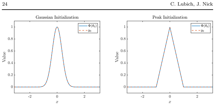
Figures from the paper (7 more)

**Figure 8.** Figure 8 [PITH_FULL_IMAGE:figures/full_fig_p025_8.png]

**Figure 8.** Figure 8 [PITH_FULL_IMAGE:figures/full_fig_p026_8.png]

**Figure 8.** Figure 8 [PITH_FULL_IMAGE:figures/full_fig_p027_8.png]

**Figure 8.** Figure 8 [PITH_FULL_IMAGE:figures/full_fig_p028_8.png]

**Figure 8.** Figure 8 [PITH_FULL_IMAGE:figures/full_fig_p029_8.png]

**Figure 8.** Figure 8 [PITH_FULL_IMAGE:figures/full_fig_p030_8.png]

**Figure 8.** Figure 8 [PITH_FULL_IMAGE:figures/full_fig_p031_8.png]

Discussion (0). Continue with ORCID to comment.

Forward citations

Cited by 2 Pith papers

Reviewed papers in the Pith corpus that reference this work. Sorted by Pith novelty score. Full citation record

Residual-Based Time Discretization on Nonlinear Approximation Manifolds: Analysis and Gaussian Applications
math.NA 2026-07 conditional novelty 6.0 of 10

Residual-minimization time steppers on nonlinear manifolds obey error bounds of order h or h² plus a residual term, with an extra conditioning term for the Dirac-Frenkel-based variant.
Dirac-Frenkel dynamics with inertia for nonlinearly parametrized solutions of evolution problems
math.NA 2026-06 unverdicted novelty 6.0 of 10

Inertial Dirac-Frenkel dynamics yield well-posed parameter evolution for nonlinear parametrizations with a posteriori error bounds and improved numerical robustness.

Reference graph

Works this paper leans on

30 extracted references · 26 canonical work pages · cited by 2 Pith papers

[1]

Anderson and M

W. Anderson and M. Farazmand. Fast and scalable computation o f shape- morphing nonlinear solutions with application to evolutional neural ne t- works. J. Comput. Phys. , 498:Paper No. 112649, 21, 2024

work page 2024
[2]

Bruna, B

J. Bruna, B. Peherstorfer, and E. Vanden-Eijnden. Neural G alerkin schemes with active learning for high-dimensional evolution equation s. J. Comput. Phys. , 496:Paper No. 112588, 22, 2024

work page 2024
[3]

J. Butcher. A stability property of implicit runge-kutta methods . BIT, 15:358–361, 1975

work page 1975
[4]

Carleo and M

G. Carleo and M. Troyer. Solving the quantum many-body problem with artiﬁcial neural networks. Science, 355(6325):602–606, 2017

work page 2017
[5]

De Ryck, F

T. De Ryck, F. Bonnet, S. Mishra, and E. de B´ ezenac. An opera tor pre- conditioning perspective on training in physics-informed machine lear ning. 32 C. Lubich, J. Nick arXiv preprint arXiv:2310.05801 , 2023

arXiv 2023
[6]

Dekker and J

K. Dekker and J. Verwer. Stability of Runge–Kutta methods for stiﬀ non- linear diﬀerential equations . North-Holland, Amsterdam, 1984

work page 1984
[7]

P. A. Dirac. Note on exchange phenomena in the Thomas atom. Proc. Cambridge Phil. Soc. , 26(3):376–385, 1930

work page 1930
[8]

Engel and R

K.-J. Engel and R. Nagel. One-Parameter Semigroups for Linear Evolu- tion Equations . Springer-Verlag, 2000

work page 2000

Show all 30 references

[9]

Feischl, C

M. Feischl, C. Lasser, C. Lubich, and J. Nick. Regularized dynamic al parametric approximation. arXiv preprint arXiv:2403.19234 , 2024

2024
[10]

Frank, J

R. Frank, J. Schneid, and C. W. Ueberhuber. Order results fo r implicit Runge–Kutta methods applied to stiﬀ systems. SIAM journal on numer- ical analysis, 22(3):515–534, 1985

1985
[11]

N. Gaby, X. Ye, and H. Zhou. Neural control of parametric so lutions for high-dimensional evolution PDEs. SIAM J. Sci. Comput. , 46(2):C155– C185, 2024

2024
[12]

D. T. Gillespie. A rigorous derivation of the chemical master equa tion. Physica A: Statistical Mechanics and its Applications , 188(1-3):404–425, 1992

1992
[13]

I. L. Guti´ errez and C. B. Mendl. Real time evolution with neura l-network quantum states. Quantum, 6:627, 2022

2022
[14]

Haegeman, J

J. Haegeman, J. I. Cirac, T. J. Osborne, I. Piˇ zorn, H. Vers chelde, and F. Verstraete. Time-dependent variational principle for quantum lattices. Physical review letters , 107(7):070601, 2011

2011
[15]

Hairer and C

E. Hairer and C. Lubich. Numerical solution of ordinary diﬀerent ial equa- tions. In The Princeton companion to applied mathematics, ed. N. J. Higham, pages 293–305. Princeton, NJ: Princeton University Press, 201 5
[16]

Hairer, S

E. Hairer, S. P. Nørsett, and G. Wanner. Solving Ordinary Diﬀerential Equations I. Nonstiﬀ Problems . Springer, Berlin, 1987

1987
[17]

Hairer and G

E. Hairer and G. Wanner. Solving Ordinary Diﬀerential Equations II. Stiﬀ and Diﬀerential-Algebraic Problems . Springer, Berlin, 1991

1991
[18]

E. J. Heller. Time dependent variational approach to semiclassic al dy- namics. The Journal of Chemical Physics , 64(1):63–73, 1976

1976
[19]

Jahnke and W

T. Jahnke and W. Huisinga. A dynamical low-rank approach to th e chemi- cal master equation. Bulletin of mathematical biology , 70:2283–2302, 2008

2008
[20]

Kaltenbacher

B. Kaltenbacher. Some newton-type methods for the regular ization of nonlinear ill-posed problems. Inverse Problems , 13(3):729, 1997

1997
[21]

Kast and J

M. Kast and J. S. Hesthaven. Positional embeddings for solving PDEs with evolutional deep neural networks. J. Comput. Phys. , 508:Paper No. 112986, 26, 2024

2024
[22]

Kramer and M

P. Kramer and M. Saraceno. Geometry of the time-dependent variational principle in quantum mechanics , volume 140 of Lecture Notes in Physics . Springer-Verlag, Berlin-New York, 1981

1981
[23]

Kvaal, C

S. Kvaal, C. Lasser, T. B. Pedersen, and L. Adamowicz. No nee d for a grid: Adaptive fully-ﬂexible gaussians for the time-dependent Schr ¨ odinger equation. arXiv preprint arXiv:2207.00271 , 2022. Regularized dynamical parametric approximation for stiﬀ p roblems 33

2022 arXiv
[24]

C. Lubich. From quantum to classical molecular dynamics: reduced mode ls and numerical analysis . European Mathematical Society, 2008

2008
[25]

Manthe, H.-D

U. Manthe, H.-D. Meyer, and L. S. Cederbaum. Wave-packet d ynamics within the multiconﬁguration Hartree framework: General aspect s and application to NOCl. The Journal of Chemical Physics , 97(5):3199–3213, 1992

1992
[26]

Schmitt and M

M. Schmitt and M. Heyl. Quantum many-body dynamics in two dimen - sions with artiﬁcial neural networks. Phys. Rev. Lett. , 125(10):100503, 7, 2020

2020
[27]

Schwerdtner, P

P. Schwerdtner, P. Schulze, J. Berman, and B. Peherstorfe r. Nonlinear embeddings for conserving Hamiltonians and other quantities with ne ural Galerkin schemes. SIAM J. Sci. Comput. , 46(5):C583–C607, 2024

2024
[28]

von Neumann

J. von Neumann. Eine Spektraltheorie f¨ ur allgemeine Operator en eines unit¨ aren Raumes.Math. Nachr. , 4:258–281, 1951

1951
[29]

Y. Wen, E. Vanden-Eijnden, and B. Peherstorfer. Coupling pa rameter and particle dynamics for adaptive sampling in neural Galerkin scheme s. Phys. D , 462:Paper No. 134129, 13, 2024

2024
[30]

Zhang, Y

H. Zhang, Y. Chen, E. Vanden-Eijnden, and B. Peherstorfer . Sequential- in-time training of nonlinear parametrizations for solving time-depen dent partial diﬀerential equations. arXiv preprint arXiv:2404.01145 , 2024

2024 arXiv

Pith tools

Reviewed August 10, 2026 · model on record in the stance chip above.

[1] [1]

Anderson and M

W. Anderson and M. Farazmand. Fast and scalable computation o f shape- morphing nonlinear solutions with application to evolutional neural ne t- works. J. Comput. Phys. , 498:Paper No. 112649, 21, 2024

work page 2024

[2] [2]

Bruna, B

J. Bruna, B. Peherstorfer, and E. Vanden-Eijnden. Neural G alerkin schemes with active learning for high-dimensional evolution equation s. J. Comput. Phys. , 496:Paper No. 112588, 22, 2024

work page 2024

[3] [3]

J. Butcher. A stability property of implicit runge-kutta methods . BIT, 15:358–361, 1975

work page 1975

[4] [4]

Carleo and M

G. Carleo and M. Troyer. Solving the quantum many-body problem with artiﬁcial neural networks. Science, 355(6325):602–606, 2017

work page 2017

[5] [5]

De Ryck, F

T. De Ryck, F. Bonnet, S. Mishra, and E. de B´ ezenac. An opera tor pre- conditioning perspective on training in physics-informed machine lear ning. 32 C. Lubich, J. Nick arXiv preprint arXiv:2310.05801 , 2023

arXiv 2023

[6] [6]

Dekker and J

K. Dekker and J. Verwer. Stability of Runge–Kutta methods for stiﬀ non- linear diﬀerential equations . North-Holland, Amsterdam, 1984

work page 1984

[7] [7]

P. A. Dirac. Note on exchange phenomena in the Thomas atom. Proc. Cambridge Phil. Soc. , 26(3):376–385, 1930

work page 1930

[8] [8]

Engel and R

K.-J. Engel and R. Nagel. One-Parameter Semigroups for Linear Evolu- tion Equations . Springer-Verlag, 2000

work page 2000