Moving-Boundary Port-Hamiltonian Systems

A. Das; S. Weiland; T.J. Meijer

REVIEW 3 major objections 4 minor 36 references

Moving-Boundary Port-Hamiltonian Systems

T0 review · 3 major / 4 minor · reviewed 2026-08-10 · deepseek-v4-flash

Challenge this review Re-run · record.json Download PDF Read on arXiv ↗ Review JSON

Pith's one-line read This paper proves that a linear port-Hamiltonian system on a time-varying spatial interval admits a time-varying Dirac structure, formally establishing moving-boundary port-Hamiltonian systems as a generalization of the fixed-domain theory.

desk verdict The moving-boundary port-Hamiltonian construction is a real contribution and likely correct when both boundary velocities are nonzero, but Theorem 1 as stated is false at instants where one velocity vanishes. read the letter →

arxiv 2501.14930 v2 pith:F7RROMH2 submitted 2025-01-24 math.OC cs.NAmath.NA

T.J. Meijer , A. Das , S. Weiland This is my paper · ORCID

classification math.OCcs.NAmath.NA MSC 37K0593C2065M5035Q93

keywords port-HamiltoniansystemsDiracstructuremovingboundaryfreeproblemsdistributedparametertransportequationspatialdiscretizationtelegrapher'sequations

verification ladder T0 review T1 audit T2 compute T3 formal

The pith

A machine-rendered reading of the paper's core claim, the machinery that carries it, and where it could break.

The reading

This paper aims to extend boundary port-Hamiltonian systems — PDE models whose energy exchange with the environment is encoded in a Dirac structure — from fixed spatial domains to domains whose endpoints move over time. The authors prove that a linear first-order port-Hamiltonian PDE on a time-varying interval $[a(t), b(t)]$ still carries a Dirac structure, provided the domain is re-parameterized onto a fixed reference interval and the boundary motion is folded into the port variables. This yields the new class of moving-boundary port-Hamiltonian systems, which reduces to the classical definition when the boundaries are stationary. The result matters because moving domains arise in phase-transition problems, deforming mechanical systems, and lithography equipment, where ignoring conservation structure is known to damage controller design and simulation. The paper also turns the structure into a dynamic-mesh spatial discretization for the telegrapher's equations and checks it numerically.

What carries the argument

The load-bearing object is the time-varying Stokes–Dirac structure $\hat D(t)$ on the fixed reference domain $\hat s \in [0,1]$, obtained by the change of spatial coordinates $s = a(t) + (b(t)-a(t))\hat s$ and the state rescaling $\hat x = \sqrt{b-a}\,x$. The coordinate change converts the moving endpoints into two new flow terms: a compression term $-\frac{1}{2}(\dot b-\dot a)/(b-a)\hat x$ and a translation term $\partial_{\hat s}\big((\dot a + (\dot b-\dot a)\hat s)/(b-a)\hat x\big)$, which the paper interprets physically and packages into the port equations (13). The proof of the Dirac property combines Stokes' theorem, which handles the internal Hamiltonian operator, with the Leibniz integral rule, which handles the moving integration bounds; the price of this packaging is that the boundary ports take complex values whenever a boundary velocity is negative, with the pairing $\hat f_\partial^H \hat e_\partial$ remaining real under Assumption 1(iii).

What would settle it

Evaluate the Dirac orthogonality condition $\hat D(t) = \hat D^\perp(t)$ symbolically for the ports (13) under $\dot a(t) < 0 < \dot b(t)$: the substitution $\sqrt{\dot a}\sqrt{\dot b} = \sqrt{\dot a\dot b}$ used in Appendix C ceases to hold over the reals, so a direct check of whether the subspace is self-orthogonal under the complex pairing settles whether Theorem 1 survives outside Assumption 1(iii).

Watch

Extended reading notes

Core claim

On the paper's own terms, the central discovery is Theorem 1: for a linear boundary port-Hamiltonian system on a time-varying interval $[a(t),b(t)]$ whose endpoints satisfy Assumption 1, the time-dependent subspace $\hat D(t)$ defined by the flow equation $\hat f = -\frac{1}{2}\frac{\dot b-\dot a}{b-a}Q^{-1}\hat e + \partial_{\hat s}\big(\frac{\dot a+(\dot b-\dot a)\hat s}{b-a}Q^{-1}\hat e\big) + \hat J(t)\hat e$ together with the port equations (13) is a Dirac structure for all $t$. From this, Proposition 3 concludes that the moving-boundary system is exactly the dynamical system $(\partial_t\hat x, \hat f_\partial, Q\hat x, \hat e_\partial) \in \hat D(t)$, a genuine generalization of the static-domain definition whose two extra flow terms correspond to compression of the domain and translation of material points through it. The power balance acquires boundary terms equal to the boundary velocity times the energy density at the boundary, and when $\dot a = \dot b = 0$ all formulas collapse to the classical Stokes-Dirac structure.

Load-bearing premise

The whole construction assumes the two boundary velocities always have the same sign (both boundaries move in the same direction), because the proof needs $\sqrt{\dot a}\sqrt{\dot b} = \sqrt{\dot a \dot b}$ to keep the port pairings real.

Editorial extensions

If this is right

When the boundary velocities vanish, Proposition 3 reduces to the standard static-domain port-Hamiltonian definition, so the new class strictly generalizes the old one.
The power balance of a moving-domain system gains the boundary power flow $\frac{1}{2}(\dot b\, \hat e^\top(1)\hat x(1) - \dot a\, \hat e^\top(0)\hat x(0))$: boundary motion itself transports energy in or out, beyond the usual port power.
For the lossless transmission line, total charge and flux in the moving segment change only through boundary terms; boundary motion acts like an extra current equal to the charge density times the boundary velocity.
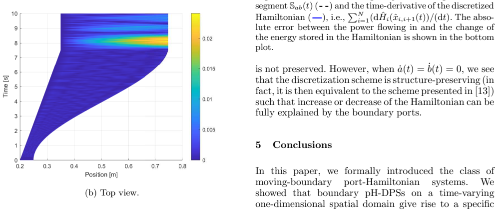
The Dirac structure yields a dynamic-grid discretization of the telegrapher's equations whose mesh tracks the moving boundaries, with numerical error that decreases as the number of elements grows.
The discretization recovers the structure-preserving scheme of [13] whenever the domain is static, and otherwise approximately preserves power balance with bounded error.

Reading between the lines

Editorial extensions of the paper, not claims the author makes directly.

A natural next step is a structure-preserving dynamic-mesh discretization: the scheme in Section 4 deliberately drops exact power balance when boundaries move, while Theorem 1 provides the discrete Dirac structure such a scheme would need to respect exactly.
The domain of validity is genuinely fixed by Assumption 1(iii): opposite-sign boundary motion (one end expanding while the other contracts) falls outside the theorem, and a different port assignment or a realification of the structure would be needed to cover it — for instance breathing domains or two-sided Stefan-like fronts moving against each other.
Because the construction is generic in the Hamiltonian operator $J = J_0 + J_1\partial_s$, the same moving-boundary treatment should apply to transport, shallow-water, and beam-type models, not only the lossless transmission line shown here.
The complex-valued ports suggest that the moving-boundary structure may be viewed as a complexified Dirac structure whose real power pairing is recovered from the boundary-velocity sign condition; making that interpretation explicit could connect the framework to para-complex or phase-field formulations of moving interfaces.

Share X Bluesky LinkedIn Reddit HN

Signed reviews

No signed human review yet.

Editorial analysis

A structured set of objections, weighed in public.

Desk editor's note, referee report, and a circularity audit.

Desk Editor's Note

read the letter

Take a look at arXiv:2501.14930. The authors extend port-Hamiltonian systems to one-dimensional domains with moving boundaries, and the first half is genuinely useful: the change of variables, the state dynamics in (8), and the power balance in (10) are clean, and they correctly identify the earlier moving-interface papers as special cases. The Dirac structure idea is the right one.

The problem is Theorem 1. As stated, it is false. Assumption 1(iii) allows one boundary velocity to be zero, and the proof of D̂⊥ ⊂ D̂ in Appendix C breaks exactly there. The step from (C.12) to the port equations requires both √ȧ and √ḃ to be nonzero; if ȧ=0, the bilinear pairing only forces a relation between φ∂2 and η∂2, not the individual port equations. Concretely, with n=1, Q=1, ȧ=0, ḃ=1, the element γ1=(φ=0, φ∂1=0, η∂1=0, φ∂2=1, η∂2=-1/2, η=0) is in D̂⊥ but violates the port equations, so D̂⊥ ≠ D̂. This is not a pathological corner: their own transmission-line example has ḃ(0)=0 and both velocities zero for t>7.5.

The fix is probably to require ȧḃ>0 strictly, or to treat zero-velocity instants with a degenerate structure separately. Either way, the paper overclaims as written. The theorem is likely correct on the open set where both boundaries move in the same direction at nonzero speed, and the construction is a real contribution. The minor issues—Assumption 1(i) says continuity but uses derivatives, and the numerical section is a single illustrative run with no convergence study or code—are secondary. The discretization honesty is a plus: they state clearly it is not structure-preserving.

I'd send this to referees; the flaw is concrete and fixable, and the result is significant enough to warrant the effort. The verdict should be revise before accept, not reject.

Referee Report

3 major / 4 minor

Summary. The paper develops a port-Hamiltonian formulation for linear boundary port-Hamiltonian distributed parameter systems on a one-dimensional time-varying interval. It introduces a normalized coordinate, derives transformed state dynamics (Lemma 2, Eq. (8)), a power balance (the second Lemma 2, Eq. (10)), and a time-varying Dirac structure (Theorem 1) with boundary ports (13), from which it defines moving-boundary port-Hamiltonian systems (Proposition 3). The framework is then applied to a dynamic-mesh discretization of the telegrapher's equations, with numerical validation. The central contribution is the Dirac-structure characterization; the discretization is presented as a consequence of that structure.

Significance. If the Dirac-structure result were correct under the stated assumptions, this would be a genuinely useful contribution: it gives a concrete, physically interpretable way to preserve power balance under moving boundaries and a principled basis for dynamic-mesh discretization. The chain-rule derivation of the dynamics and the energy-balance computation are transparent, and the telegrapher example is well chosen. The authors also deserve credit for explicitly constructing time-varying ports and for reporting the non-preservation of the discretized power balance rather than hiding it. However, the main theorem is not correct as stated: the proof degenerates at instants where one boundary velocity vanishes, and Assumption 1 as written also allows cases not covered by the square-root identities used in the proof. The significance of the paper therefore depends on repairing this degeneracy and clarifying the admissible velocity regimes.

major comments (3)

[Theorem 1 and Appendix C, Eq. (C.12)] The Dirac-structure claim fails when one boundary velocity vanishes, which is allowed by Assumption 1(iii). The final step of the proof infers the second-block port equations from Eq. (C.12), but if, say, a_dot(t)=0 and b_dot(t)>0, Eq. (C.12) yields only a one-dimensional relation and does not imply the two port equalities in (13). A concrete counterexample is n=1, Q=1, a_dot=0, b_dot=1, and the element gamma1 = (phi=0, phi_d1=0, eta_d1=0, phi_d2=1, eta_d2=-1/2, eta=0). For every element gamma=(f, f_d, e, e_d) in D_hat(t), the second-block port equations give e_d2 = (1/2) f_d2, so the pairing of gamma1 with gamma vanishes; hence gamma1 is in D_hat(t)^perp. But gamma1 does not satisfy the port equations of (13), so gamma1 is not in D_hat(t). Thus D_hat(t)^perp is strictly larger than D_hat(t). This is not a remote corner case: in the numerical example of Section 4.2, b_dot(0)=0 and both velocities are zero for t>7.5. The theorem should either assume strictly nonzero velocities of the same sign and treat static instants separately, or the port construction must be modified to remove the degeneracy. As stated, the central claim is false.
[Assumption 1(i), Lemma 2, Theorem 1] Assumption 1(i) states only that a,b are continuous, but the entire derivation differentiates them: Eq. (8), Theorem 1, and the boundary-port definition (13) all use a_dot and b_dot. The assumption should be C^1, or piecewise C^1 with the theorem stated on each differentiability interval. Moreover, the numerical example in Section 4.2 defines b(t) piecewise with a jump in b_dot at t=7.5; as written, the theorem is asserted at that instant even though the boundary velocity is not defined there. This is a load-bearing regularity gap, not merely a presentation issue.
[Appendix C, Eqs. (C.3) and (C.11)] The proof uses the identity sqrt(a_dot) sqrt(b_dot) = sqrt(a_dot b_dot). With the standard principal branch this identity holds only when both velocities are nonnegative. Assumption 1(iii) as written also permits a_dot<0 and b_dot<0, for which sqrt(a_dot) sqrt(b_dot) = -sqrt(a_dot b_dot). If the intended scope is expanding or contracting domains with nonnegative velocities, Assumption 1(iii) must be replaced by a_dot, b_dot >= 0; otherwise the proof must specify a branch convention and handle the sign. As stated, the Dirac-structure proof does not cover the full range of Assumption 1.

minor comments (4)

[Section 3.3] The power-balance result is also labelled Lemma 2, duplicating the dynamics lemma of Section 3.1; the second one should be renumbered and cross-references updated.
[Section 3.2] The definition of phi_hat(t, s_hat) appears to omit the factor sqrt(b(t)-a(t)): it is written as phi(t, h(t, s_hat)), while Eq. (4) applies the factor to all components of x. This is inconsistent with the Hamiltonian scaling and with the energy-balance expressions that follow.
[Section 3.5.2 and Theorem 1] In Eq. (13), the sentence about z denoting the complex conjugate of z is unclear because no overlines appear in the displayed matrix. It should be stated explicitly which entries involving sqrt(a_dot) and sqrt(b_dot) are conjugated, and for negative velocities the branch of the square root must be specified.
[Theorem 1 statement] The set comprehension in Theorem 1 has a typo: it should read (f_hat, f_d_hat, e_hat, e_d_hat) in B_hat(t), not (f_hat, f_d_hat, e_hat, e_d_hat in B_hat(t)).

Circularity Check

0 steps flagged · score 0.0 of 10

No significant circularity: the moving-boundary Dirac structure is proved from the independent static Stokes–Dirac structure, and the boundary ports are an explicit construction, not a fitted prediction.

full rationale

The paper's central claim is that the subspace D̂(t) defined in Theorem 1 is a Dirac structure. Appendix C proves both inclusions D̂(t) ⊂ D̂⊥(t) and D̂⊥(t) ⊂ D̂(t) by direct computation: the internal-dynamics terms are reduced, via integration by parts, to the static Stokes–Dirac identity (C.1) imported from Villegas' Lemma 1, and the moving-boundary terms are handled by factoring the boundary expression under Assumption 1(iii). The boundary ports in (13) are introduced explicitly so that the previously derived power balance (10) reads ⟨f̂,ê⟩ = ⟨f̂∂,ê∂⟩; this is a construction/ansatz step, not a fitted parameter later relabeled as a prediction. Proposition 3 packages the dynamics already derived in Lemma 2 into the pH membership statement (14), but the nontrivial content is the theorem that D̂(t) is a Dirac structure, which is proved rather than assumed. The paper's self-citations (Meijer's thesis [25], Voß–Weiland [35]) appear only as background and are not load-bearing. Concerns about Assumption 1(iii), zero boundary velocities, and the gap between continuity and differentiability in Assumption 1(i) are correctness or well-posedness issues, not circularity, and therefore do not raise the circularity score.

Assumptions & free parameters 0 free parameters · 4 assumptions · 0 invented entities

The central claim depends on the cited static Dirac structure, the boundary regularity and same-direction-motion assumption, and the formal complexification of Dirac structures. No free parameters are fitted and no new physical entities are introduced.

assumptions (4)

standard math Static Stokes-Dirac structure (Lemma 1, from Villegas 2007) exists for J = J0 + J1∂s with boundary ports parameterized by S1 and M.
The moving-boundary Dirac structure is built on this known result; the paper uses it in the proof of Lemma 2 and Theorem 1 without re-deriving it.
domain assumption Assumption 1: a, b continuous with a(t) < b(t) and ȧ(t)ḃ(t) ≥ 0 for all t.
The continuity statement is weaker than the differentiability actually used in the derivation; the same-direction condition is load-bearing in the proof of Theorem 1 (Appendix C, Eqs. C.3 and C.11).
domain assumption Sufficient regularity of the state x and the boundary traces for the chain rule and integration by parts on L2([a,b]).
The dynamics derivation in Appendix A and the Dirac proof in Appendix C move derivatives between x, e, and traces without a precise function-space setup.
standard math Definition of Dirac structures over K = C with non-degenerate bilinear form (allowed by Jeltsema and van der Schaft).
Needed to allow complex-valued port variables when boundary velocities are negative; Assumption 1(iii) keeps the power real.

how reviews work

0 comments

Cite this review

Pith. "Pith review of Moving-Boundary Port-Hamiltonian Systems." pith.science (2026). https://pith.science/paper/F7RROMH2

@misc{pith2026250114930,
  author       = {Pith},
  title        = {Pith review of: Moving-Boundary Port-Hamiltonian Systems},
  year         = {2026},
  howpublished = {\url{https://pith.science/paper/F7RROMH2}},
  note         = {Machine review of arXiv:2501.14930}
}

read the original abstract

In this paper, we consider linear boundary port-Hamiltonian distributed parameter systems on a time-varying spatial domain. We derive the specific time-varying Dirac structure that these systems give rise to and use it to formally establish a new class of moving-boundary port-Hamiltonian systems by showing that these distributed parameter systems on a time-varying spatial domain admit a port-Hamiltonian representation. We demonstrate that our results can be leveraged to develop a spatial discretization scheme with dynamic meshing for approximating the telegrapher's equations on a time-varying spatial domain, which we subsequently verify numerically.

Figures

Figures reproduced from arXiv: 2501.14930 by the authors.

**Figure 2.** Simulated voltage ( ) in the time-varying segment Sab(t) ( ). Outside Sab(t), the analytic solution Vtrue ( ) is depicted. segment given by Sab(t) = [2 + 0.2t, 5 − cos(0.25t)]/10, for t 6 t,¯ [2 + 0.2t,¯ 5 − cos(0.25t¯)]/10, for t > t,¯ where t¯ = 7.5 s. In other words, a(t) = 0.2 + 0.02t and b(t) = 0.5 − 0.25 cos(0.25t) for t ∈ [0, 7.5] after which the boundaries remain static at a(7.5) and b(7.5). We use the di… view at source ↗

**Figure 4.** Power balance showing the power flowing into the TL [PITH_FULL_IMAGE:figures/full_fig_p010_4.png] view at source ↗

Figures from the paper (1 more)

**Figure 3.** Figure 3: Absolute value of the error with respect to the analyt [PITH_FULL_IMAGE:figures/full_fig_p010_3.png]

Discussion (0). Continue with ORCID to comment.

Reference graph

Works this paper leans on

36 extracted references · 35 canonical work pages

[1]

Augner and H

B. Augner and H. Laasri. Exponential stability for inﬁni te- dimensional non-autonomous port-Hamiltonian systems. Syst. Control Lett. , 144:104757, 2020

work page 2020
[2]

Baaiu, F

A. Baaiu, F. Couenne, D. Eberard, C. Jallut, L. Lefevre, Y. Legorrec, and B. Maschke. Port-based modelling of mass transport phenomena. Math. Comput. Model. Dyn. Syst. , 15(3):233–254, 2009

work page 2009
[3]

Beattie, V

C. Beattie, V. Mehrmann, H. Xu, and H. Zwart. Linear port-Hamiltonian descriptor systems. Math. Control, Signals, Syst., 30(17):1–27, 2018. 10

work page 2018
[4]

Breiten and B

T. Breiten and B. Unger. Passivity preserving model reduction via spectral factorization. Automatica, 142:110368, 2022

work page 2022
[5]

Brugnoli, R

A. Brugnoli, R. Rashad, and S. Stramigioli. Dual ﬁeld structure-preserving discretization of port-Hamilt onian systems using ﬁnite element exterior calculus. J. Comput. Phys., 471:111601, 2022

work page 2022
[6]

H. Butler. Position control in lithography equipment. IEEE Control Syst. Mag. , 31(5):28–47, 2011

work page 2011
[7]

Califano, A

F. Califano, A. Dijkshoorn, S. Roodink, and S. Stramigio li. Energy-aware control of Euler-Bernoulli beams by means of an axial load. IEEE ASME Trans. Mechatron. , 27(6):5959– 5968, 2022

work page 2022
[8]

G. F. Carey and D. L. Humphrey. Mesh reﬁnement and iterative solution methods for ﬁnite element computations . Int. J. Numer. Methods Eng. , 17(11):1717–1734, 1981

work page 1981

Show all 36 references

[9]

T. J. Courant and A. W einstein. Beyond Poisson structure s. S´ eminaire Sud-Rhodanien de G´ eometrie, 8, 1988

1988
[10]

Diagne and B

M. Diagne and B. Maschke. Port Hamiltonian formulation of a system of two conservation laws with a moving interface. Eur. J. Control , 19:495–504, 2013

2013
[11]

Duindam, A

V. Duindam, A. Macchelli, S. Stramigioli, and H. Bruyni nckx. Modeling and control of complex physical systems: The port- Hamiltonian approach. Springer, 2014

2014
[12]

Gibou and R

F. Gibou and R. Fedkiw. A fourth order accurate discretization for the Laplace and heat equations on arbitr ary domains, with applications to the Stefan problem. J. Comput. Phys., 202(2):577–601, 2005

2005
[13]

G. Golo, V. Talasila, A. van der Schaft, and B. Maschke. Hamiltonian discretization of boundary control systems. Automatica, 40(5):757–771, 2004

2004
[14]

Gugercin, R

S. Gugercin, R. V. Polyuga, C. Beattie, and A. van der Schaft. Structure-preserving tangential interpolation f or model reduction of port-Hamiltonian systems. Automatica, 48(9), 2012

2012
[15]

Hamroun, A

B. Hamroun, A. Dimofte, L. Lef` evre, and E. Mendes. Control by interconnection and energy-shaping methods of port Hamiltonian models. Application to the shallow water equations. Eur. J. Control , 16(5):545–563, 2010

2010
[16]

Hamroun, L

H. Hamroun, L. Lef` evre, and E. Mendes. Port-based modelling for open channel irrigation systems. Trans. Fluid Mech., 1(12):995–1009, 2006

2006
[17]

Jacob and H

B. Jacob and H. J. Zwart. Linear port-Hamiltonian systems on inﬁnite-dimensional spaces , volume 223 of Operator theory: Advances and applications . Spinger, 2012

2012
[18]

Jeltsema and A

D. Jeltsema and A. van der Schaft. Complexiﬁcation of Dirac structures and generalized Kirchhoﬀ operators. IF AC- PapersOnLine, 48(13):75–80, 2015

2015
[19]

Kilian, B

A. Kilian, B. Maschke, A. Mironchenko, and F. Wirth. A ca se study of port-Hamiltonian systems with a moving interface. IEEE Control Syst. Lett. , 7:1572–1577, 2023

2023
[20]

Le Gorrec, H

Y. Le Gorrec, H. Zwart, and B. Maschke. Dirac structures and boundary control systems associated with skew-symmetric diﬀerential operators. SIAM J. Control Opt. , 44(5):1864– 1892, 2005

2005
[21]

D. Lou. Parameterized model order reduction with applications to thermal systems . PhD thesis, Eindhoven University of Technology, 2021

2021
[22]

Macchelli and F

A. Macchelli and F. Califano. Dissipativity-based bou ndary control of linear distributed port-Hamiltonian systems. Automatica, 95:54–62, 2018

2018
[23]

Maschke and A

B. Maschke and A. van der Schaft. Linear boundary port- Hamiltonian systems with implicitly deﬁned energy, 2023. preprint: https://arxiv.org/abs/2305.13772

2023 arXiv
[24]

Mehrmann and R

V. Mehrmann and R. Morandin. Structure-preserving discretization of port-Hamiltonian descriptor systems. I n 58th IEEE Conf. Decis. Control , pages 6863–6868, 2019

2019
[25]

T. J. Meijer. Estimation and control for discrete-time parameter-varying and descriptor systems . PhD thesis, Eindhoven University of Technology, 2024

2024
[26]

M. H. Protter and C. B. Morrey. Intermediate calculus , chapter 8. Springer, 1985

1985
[27]

D. Rees. Basic engineering plasticity: An introduction with engineering and manufacturing applications . Elsevier, 2012

2012
[28]

L. I. Rubinshte ˘in. The Stefan problem . American Mathematical Society, 1971

1971
[29]

Schwerdtner, T

P. Schwerdtner, T. Moser, V. Mehrmann, and M. Voigt. Optimization-based model order reduction of port- Hamiltonian descriptor systems. Syst. Control Lett. , 182:105655, 2023

2023
[30]

van den Hurk

D. van den Hurk. Active wafer clamp control of wafer heating eﬀects in extreme ultraviolet lithography . PhD thesis, Technische Universiteit Eindhoven, 2020

2020
[31]

A. J. van der Schaft and B. M. Maschke. Hamiltonian formulation of distributed-parameter systems with bounda ry energy ﬂow. J. Geom. Phys. , 42(1-2):166–194, 2002

2002
[32]

D. W. M. Veldman. Modeling and control of thermomechanical systems: Managing heat- induced deformation in extreme ultraviolet lithography . PhD thesis, Eindhoven University of Technology, 2020

2020
[33]

J. A. Villegas. A port-Hamiltonian approach to distributed parameter systems. PhD thesis, University of Twente, 2007

2007
[34]

Vincent, F

B. Vincent, F. Couenne, and B. Maschke L. Lef` evre. Port Hamiltonian systems with moving interface: A phase ﬁeld approach. IF AC-PapersOnLine, 53(2):7569–7574, 2020

2020
[35]

Voß and S

T. Voß and S. W eiland. Structure preserving spatial discretization of 1D convection-diﬀusion port-Hamiltoni an systems. In 50th IEEE Conf. Decis. Control , pages 6979– 6984, 2011

2011
[36]

W ang, A

M. W ang, A. Bestler, and P. Kotyczka. Modeling, discretization and motion control of a ﬂexible beam in the port-Hamiltonian framework. IF AC-PapersOnLine, 50(1):6799–6806, 2017. Appendix A Proof of Lemma 2 We will now derive the dynamics that govern ˆ x ∈ ˆX (t), t ∈ T. To th...

2017

Pith tools

Reviewed August 10, 2026 · model on record in the stance chip above.

[1] [1]

Augner and H

B. Augner and H. Laasri. Exponential stability for inﬁni te- dimensional non-autonomous port-Hamiltonian systems. Syst. Control Lett. , 144:104757, 2020

work page 2020

[2] [2]

Baaiu, F

A. Baaiu, F. Couenne, D. Eberard, C. Jallut, L. Lefevre, Y. Legorrec, and B. Maschke. Port-based modelling of mass transport phenomena. Math. Comput. Model. Dyn. Syst. , 15(3):233–254, 2009

work page 2009

[3] [3]

Beattie, V

C. Beattie, V. Mehrmann, H. Xu, and H. Zwart. Linear port-Hamiltonian descriptor systems. Math. Control, Signals, Syst., 30(17):1–27, 2018. 10

work page 2018

[4] [4]

Breiten and B

T. Breiten and B. Unger. Passivity preserving model reduction via spectral factorization. Automatica, 142:110368, 2022

work page 2022

[5] [5]

Brugnoli, R

A. Brugnoli, R. Rashad, and S. Stramigioli. Dual ﬁeld structure-preserving discretization of port-Hamilt onian systems using ﬁnite element exterior calculus. J. Comput. Phys., 471:111601, 2022

work page 2022

[6] [6]

H. Butler. Position control in lithography equipment. IEEE Control Syst. Mag. , 31(5):28–47, 2011

work page 2011

[7] [7]

Califano, A

F. Califano, A. Dijkshoorn, S. Roodink, and S. Stramigio li. Energy-aware control of Euler-Bernoulli beams by means of an axial load. IEEE ASME Trans. Mechatron. , 27(6):5959– 5968, 2022

work page 2022

[8] [8]

G. F. Carey and D. L. Humphrey. Mesh reﬁnement and iterative solution methods for ﬁnite element computations . Int. J. Numer. Methods Eng. , 17(11):1717–1734, 1981

work page 1981