REVIEW 3 major objections 5 minor 3 cited by
Adaptive kernel predictors from feature-learning infinite limits of neural networks
T0 review · 3 major / 5 minor · reviewed 2026-08-08 · deepseek-v4-flash
Pith's one-line read Infinitely wide feature-learning neural networks are kernel machines with data-dependent kernels.
desk verdict A serious theory paper with a genuinely new aNBK construction and a real gap in the aNTK claim: Appendix F.2 concedes the fixed-point equations don't determine the kernel. read the letter →
The pith
A machine-rendered reading of the paper's core claim, the machinery that carries it, and where it could break.
The reading
What carries the argument
The carrying objects are two data-dependent kernel matrices and the equations that determine them. For aNBK, the layer feature kernels $\Phi^\ell_{\mu\nu}=N^{-1}\phi(h^\ell_\mu)\cdot\phi(h^\ell_\nu)$ and their conjugate dual kernels $\widehat{\Phi}^\ell$ are fixed by the saddle point of the Bayesian action $S=-\frac12\sum_{\ell=1}^L\mathrm{Tr}(\Phi^\ell\widehat{\Phi}^\ell)+\frac{\gamma_0^2}{2}y^\top(\beta^{-1}I+\Phi^L/\lambda_L)^{-1}y-\sum_{\ell=1}^{L-1}\ln Z^\ell[\Phi^{\ell-1},\widehat{\Phi}^\ell]$, a min-max problem whose solution is the kernel in Eq. (5). For aNTK, the machinery is the DMFT field dynamics for pre-activations $h^\ell_\mu(t)$ and pre-gradient signals $z^\ell_\mu(t)$; with weight decay the initial-condition noise is exponentially suppressed, and the infinite-time fixed point of these fields defines $K_{\mathrm{aNTK}}=\lim_{t\to\infty}\sum_{\ell}G^{\ell+1}_{\mu\nu}(t,t)\Phi^\ell_{\mu\nu}(t,t)$ in Eq. (11). These objects are what make the infinite-width limit a kernel machine: they convert the training data and task labels into a kernel without perturbing $\gamma_0$.
What would settle it
Train two very wide two-layer ReLU networks with the same data, loss, and hyperparameters but different initial weight distributions (Gaussian versus Laplace) in the rich regime with weight decay; if the converged predictors differ at large width, then $K_{\mathrm{aNTK}}$ depends on training history rather than being a deterministic data-dependent kernel.
Extended reading notes
Core claim
The central discovery is that infinitely wide MLPs and CNNs trained in the rich, feature-learning regime (maximal-update parameterization, $\gamma_0=\Theta(1)$) converge to kernel regressors with data-dependent kernels. In the Bayesian setting, taking $t\to\infty$ at fixed temperature and then $N\to\infty$ gives $f_{\mathrm{aNBK}}(x)=\Phi_L(x)^\top(\Phi_L+\lambda_L I/\beta)^{-1}y$, where $\Phi_L$ is the converged last-layer feature kernel obtained from the min-max saddle point of the action $S(\{\Phi^\ell,\widehat{\Phi}^\ell\})$ in Eq. (6). In the gradient-flow setting, taking $N\to\infty$ and then $\beta\to\infty$ with weight decay $\lambda>0$ gives $f_{\mathrm{aNTK}}(x)=k_{\mathrm{aNTK}}(x)^\top(K_{\mathrm{aNTK}}+\lambda L\kappa I)^{-1}y$, where $K_{\mathrm{aNTK}}$ is the infinite-time limit of the DMFT kernel dynamics. These kernels are deterministic functions of the data and hyperparameters, recoverable numerically without expanding in the richness parameter $\gamma_0$; when $\gamma_0\to0$ they reduce to the NNGP and NTK predictors. The paper also solves the deep linear case exactly, obtaining layerwise kernel-label overlap recursions and scaling laws, and shows numerically that the adaptive kernels match finite-width trained networks and achieve lower test loss than lazy kernels on CIFAR10 and MNIST.
Load-bearing premise
The argument assumes that infinitely wide training settles into a unique final state whose kernel is purely a function of the data and training settings; the appendix notes the equations fix only the first two moments of the neuron's pre-activation distribution, so the full distribution—and hence the kernel—may still depend on how training started.
Editorial extensions
If this is right
- At $\gamma_0\to0$, the aNBK and aNTK predictors reduce to the NNGP and NTK kernels, so lazy kernel theory is the weak-feature-learning edge of a single adaptive-kernel family.
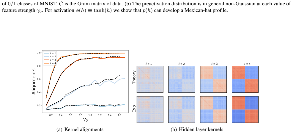
- Feature learning at infinite width produces non-Gaussian pre-activation densities and label-aligned layer kernels; these are directly computable from the saddle-point or DMFT solutions, so kernel regression with adaptive kernels inherits them.
- The aNBK and aNTK predictors can be evaluated numerically (Algorithms 1 and 2) and match finite-width trained networks at widths such as $N=5000$ on CIFAR10, making them candidate stand-ins for actual rich training.
- For deep linear networks with whitened data, the kernel-label overlaps $c_\ell$ grow exponentially in layer depth, so alignment with labels propagates from the last layer backward; the scaling laws $c_L\sim 1+L\gamma_0^2$, $c_L\sim\gamma_0^{2L/(L+1)}$, and $c_L\sim L\gamma_0^2/\ln(L\gamma_0^2)$ characterize the lazy, rich-shallow, and deep limits.
Reading between the lines
- The paper does not say this, but if the aNTK claim holds, weight decay is not just regularization: it is the mechanism that erases initialization memory and makes the infinite-width limit a history-independent kernel machine, which suggests that tuning $\lambda$ controls how kernel-like a trained network is and that at $\lambda=0$ no kernel representation of the converged predictor should be expec
- Because Appendix F.2 reports that the DMFT fixed-point equations fix only the first two moments of the single-site density and the full marginal remains history dependent, the aNTK kernel defined in Eq. (11) may not be unique unless additional conditions select a density; an extension would be to identify those extra fixed-point constraints or characterize the basin of densities.
- One testable extension is to use the adaptive kernels as cheap surrogates for feature-learning networks in scaling-law studies: if the kernel predictor matches finite-width training at moderate $N$, it could replace expensive runs when predicting scaling exponents.
- The min-max solver's convergence difficulty for $L>1$ (helped by warm starts in Fig. 4) suggests that proving convergence or finding a convex reformulation of Eq. (8) would be needed before aNBK can serve as a drop-in training surrogate for deep architectures.
Editorial analysis
A structured set of objections, weighed in public.
Referee Report
Summary. The paper studies infinite-width limits of neural networks in the feature-learning (maximal-update) regime and claims that, in two settings, the learned predictor is a kernel machine with a data-dependent kernel. The first setting is infinite-time noisy gradient flow at fixed temperature: the authors derive a statistical-mechanics action whose saddle point leads to a min-max problem for layer feature kernels and dual kernels, yielding the aNBK predictor (Eq. 5). The second setting is infinite-time gradient flow with weight decay: using DMFT equations imported from Bordelon and Pehlevan (2022), the authors define the aNTK predictor (Eq. 11) in terms of fixed-point feature and gradient kernels. The paper solves the deep linear case exactly, provides numerical algorithms for the nonlinear case, and compares the resulting predictors against finite-width MLP and CNN simulations, reporting that the adaptive kernels outperform NNGP and NTK predictors.
Significance. If the central claims hold, this is a significant conceptual advance: it extends the kernel-machine description of infinite-width neural networks beyond the lazy regime, giving explicit data-dependent kernels that can in principle be computed without simulating finite-width networks. The paper's strengths are its explicit predictor formulas, the exact solution and scaling laws for deep linear networks, the concrete numerical algorithms, and the careful finite-width comparisons. The main open gap, namely whether the aNTK fixed-point equations uniquely determine the kernel, does not diminish the interest of the results, but it must be resolved or clearly scoped before the abstract's claim is justified.
major comments (3)
- [Appendix F.2 / Eq. (11)] The aNTK representer theorem is not yet established because the fixed-point equations of the DMFT do not, in general, determine the kernel. Appendix F.2 states that the constraints (81) fix only the first two moments of the single-site pre-activation density and that the full marginal 'remains history dependent'; one 'has to track the entire update dynamics in order to get the full description.' For nonlinear activations, K_aNTK in Eq. (12) averages nonlinear functionals of this density, such as <phi(h)phi(h)> and <phi'(h)z phi'(h)z>, so knowledge of the first two moments is insufficient to determine K_aNTK. The F.2 linear example does not resolve this, since for linear activations the kernel depends only on the second moment. The authors should either prove that the invariant measure, or at least the kernel averages, is unique for the activations and architectures considered, or demonstrate numerically that K_aNTK is independent of the initialization and training trajectory.
- [§3.1, Eq. (8); Algorithm 1] The aNBK derivation replaces the N-to-infinity partition function by the saddle point of the action S in Eq. (8) and identifies this with a global min-max problem, but no argument is given for uniqueness, convexity-concavity, or the dominance of a global saddle point. This is not a purely formal point: the numerical solver is reported in Section 5 and Appendix G.2 to converge with difficulty for L>1, and Figure 7 was produced by initializing the solver with the empirical kernels obtained from Langevin simulations. Such a warm start can select a nearby local fixed point, so the reported agreement between theory and experiment does not yet certify Eq. (8) as a data-only predictor. Please report convergence from lazy or random initializations for the comparisons, or explicitly restrict the claims to locally stable saddle points.
- [§3.2, Eq. (13) and Eq. (14)] The derivation of Eq. (11) treats the final K_aNTK as a fixed matrix at the DMFT fixed point, but Eq. (13) shows that the feature and gradient kernels evolve along a non-Markovian trajectory whose integral terms depend on the full history of the error signal. Exponential suppression of the initial-condition terms addresses only one source of history dependence; Appendix F.2 shows that another source persists even at the fixed point. A closure argument is needed to show that the fixed-point conditions (81), together with the predictor equation, select a unique K_aNTK for each dataset and hyperparameter setting. Without such an argument, Eq. (11) is a trajectory-dependent description rather than a representer theorem with a data-dependent kernel fixed by the DMFT fixed point.
minor comments (5)
- [Eq. (13)] The notation ẍφ(h^ℓ_ν(t′)) is used without defining whether the derivative is with respect to the argument or with respect to time; please clarify.
- [Fig. 3] The caption lists the green curve as NNGPK and the orange and red curves as aNTK and aNBK, but the legend colors in the figure are not self-evident from the text; please harmonize the caption with the actual color coding.
- [Table 1] The table of limiting orders is difficult to read because the column entries are compressed; please reformat so that the order of limits for NNGPK, aNBK, NTK, and aNTK is unambiguous.
- [Appendix G.6] The complexity comparison between the theory solver and finite-width training is asymptotic only; for the reported values N=1024, P up to 1000, and T=20000, wall-clock times would be more informative than the statement that the theory solver is 'typically much lower' in cost.
- [General] The paper would benefit from a code/data availability statement; the hyperparameter details in Appendix G are helpful but not sufficient for exact reproduction of the kernel alignment numbers.
Circularity Check
Localized circularity in Fig. 7 warm start; central kernel-predictor derivations are self-contained, with the aNTK fixed-point gap flagged as a non-circular correctness risk.
-
fitted input called prediction
[Appendix A.1 (warm-start paragraph for Fig. 7)]
"However, an easier strategy for convergence is to initialize the solver Algorithm 1 with the empirical NN kernels{Φℓ}Lℓ=1 at convergence obtained from Langevin simulations and perturbed with a multiplicative Gaussian noise. In this way, one only needs to solve for the dual variables. This warm start allows faster convergence. This is what we did to produce Fig. 7."
The theoretical curves labeled 'theory' in Fig. 7 are generated by seeding Algorithm 1 with the empirical per-layer kernels Φℓ measured from the very Langevin simulations they are meant to predict, perturbed only by multiplicative Gaussian noise, and then solving only for the dual variables Φ̂ℓ. Since the reported quantities—the kernel-label alignments A(Φℓ, yy^T) and the layer kernels themselves—are dominated by the initialized Φℓ, the agreement between theory and experiment in Fig. 7 is partly true by construction. The solver is not independently predicting the learned kernels; it is returning a nearby fixed point of the action reached from the empirical kernels, so this specific 'prediction' reduces to the empirical input plus a local relaxation.
full rationale
The paper's central claims—the aNBK predictor of Eq. (5) from the saddle point of the Bayesian posterior and the aNTK predictor of Eq. (11) from DMFT fixed points—are derivations rather than definitions: the hyperparameters {γ0, β, λ} are inputs, and the kernels are solved from self-consistent equations, so the main derivation chain is not circular. The one concrete circular step is in Appendix A.1: to produce Fig. 7, the aNBK solver is initialized with the empirical layer kernels from the Langevin simulations that the theory is supposed to reproduce. With Φℓ fixed (up to multiplicative noise) at the empirical values, the solver only adjusts the dual variables, so the reported agreement of kernel alignments and layer kernels is substantially inherited from the initialization rather than independently predicted. This is a fitted-input-called-prediction pattern, though it is confined to one numerical comparison and does not invalidate the analytic derivation by itself. Separately, the aNTK fixed-point underdetermination admitted in Appendix F.2 is a real load-bearing gap: the constraints fix only the first two moments, while the kernel averages in Eq. (12) require the full joint density, so K_aNTK may be history-dependent and not a data-only kernel. I do not count this as circularity because it is a missing uniqueness or closure argument, not an equivalence of the predictor to its inputs by construction. The DMFT citation to Bordelon and Pehlevan (2022) is same-group but is prior derivational work, not a self-citation used to forbid alternatives, so it does not raise the circularity score.
Assumptions & free parameters
free parameters (3)
- gamma0 (feature-learning strength) =
0.3 for Fig. 3; 0.2-4.0 for Figs. 10-11; 0.5-10 for Fig. 2
- lambda (weight decay / ridge) =
1.0 for MLPs; 0.01 for CNN comparisons
- beta (inverse temperature) =
infinity for aNTK; 50 for aNBK Langevin experiments
assumptions (7)
- standard math Saddle point / Laplace evaluation of the Bayesian action S at N->infinity
- domain assumption DMFT field equations (13) exactly describe infinite-width gradient flow dynamics
- domain assumption Langevin dynamics (3) samples the Gibbs posterior (9) at stationarity
- domain assumption Activation homogeneity (degree kappa) for the aNTK weight-decay fixed point
- domain assumption sigma'(s_mu) != 0 for all patterns in the aNTK derivation
- domain assumption P = Theta(1) with N->infinity, and finite N ~ 10^3-5000 captures the limit
- domain assumption The aNTK fixed point determines the kernel predictor
invented entities (3)
-
Adaptive Bayesian kernel PhiL (aNBK)
independent evidence
-
Adaptive tangent kernel K_aNTK
independent evidence
-
Dual kernels hatPhi_l
Cite this review
Pith. "Pith review of Adaptive kernel predictors from feature-learning infinite limits of neural networks." pith.science (2026). https://pith.science/paper/JCMSLQ5G
@misc{pith2026250207998,
  author       = {Pith},
  title        = {Pith review of: Adaptive kernel predictors from feature-learning infinite limits of neural networks},
  year         = {2026},
  howpublished = {\url{https://pith.science/paper/JCMSLQ5G}},
  note         = {Machine review of arXiv:2502.07998}
}
read the original abstract
Previous influential work showed that infinite width limits of neural networks in the lazy training regime are described by kernel machines. Here, we show that neural networks trained in the rich, feature learning infinite-width regime in two different settings are also described by kernel machines, but with data-dependent kernels. For both cases, we provide explicit expressions for the kernel predictors and prescriptions to numerically calculate them. To derive the first predictor, we study the large-width limit of feature-learning Bayesian networks, showing how feature learning leads to task-relevant adaptation of layer kernels and preactivation densities. The saddle point equations governing this limit result in a min-max optimization problem that defines the kernel predictor. To derive the second predictor, we study gradient flow training of randomly initialized networks trained with weight decay in the infinite-width limit using dynamical mean field theory (DMFT). The fixed point equations of the arising DMFT defines the task-adapted internal representations and the kernel predictor. We compare our kernel predictors to kernels derived from lazy regime and demonstrate that our adaptive kernels achieve lower test loss on benchmark datasets.
Figures


Figures from the paper (11 more)




Forward citations
Cited by 3 Pith papers
-
Statistical physics of deep learning: Optimal learning of a multi-layer perceptron near interpolation
A replica/HCIZ theory predicts the Bayes-optimal generalization error of proportional-width MLPs near interpolation and discovers layer-wise specialization transitions that make deeper targets harder to learn.
-
Width-Robust Learnability in Mean-Field Bayesian Neural Networks
For fixed-depth mean-field Bayesian nets on the Boolean cube, poly-sample learnability at infinite width equals poly-width learnability equals poly-bounded reduced entropy.
-
Dynamics of neural scaling laws in random feature regression with powerlaw-distributed kernel eigenvalues
A single dynamical mean-field theory unifies Bayesian, gradient-flow, and Langevin training of random-feature regression and explains finite-time generalization error on power-law spectra.
Reference graph
Works this paper leans on
-
[1]
Advani, M. S. and Saxe, A. M. High-dimensional dynamics of generalization error in neural networks, 2017. URL https://arxiv.org/abs/1710.03667
arXiv 2017
-
[2]
Why bigger is not always better: on finite and infinite neural networks
Aitchison, L. Why bigger is not always better: on finite and infinite neural networks, 2020. URL https://arxiv.org/abs/1910.08013
work page Pith review arXiv 2020
-
[3]
Aiudi, R., Pacelli, R., Vezzani, A., Burioni, R., and Rotondo, P. Local kernel renormalization as a mechanism for feature learning in overparametrized convolutional neural networks. Nature Communications, 16, 2023. URL https://api.semanticscholar.org/CorpusID:260125263
work page 2023
-
[4]
A convergence analysis of gradient descent for deep linear neural networks, 2019 a
Arora, S., Cohen, N., Golowich, N., and Hu, W. A convergence analysis of gradient descent for deep linear neural networks, 2019 a . URL https://arxiv.org/abs/1810.02281
arXiv 2019
-
[5]
S., Hu, W., Li, Z., Salakhutdinov, R., and Wang, R
Arora, S., Du, S. S., Hu, W., Li, Z., Salakhutdinov, R., and Wang, R. On exact computation with an infinitely wide neural net, 2019 b . URL https://arxiv.org/abs/1904.11955
arXiv 2019
-
[6]
Cugliandolo-Kurchan equations for dynamics of Spin-Glasses
Arous, G. B., Dembo, A., and Guionnet, A. Cugliandolo-kurchan equations for dynamics of spin-glasses, 2004. URL https://arxiv.org/abs/math/0409273
work page Pith review arXiv 2004
-
[7]
Neural networks as kernel learners: The silent alignment effect, 2021
Atanasov, A., Bordelon, B., and Pehlevan, C. Neural networks as kernel learners: The silent alignment effect, 2021. URL https://arxiv.org/abs/2111.00034
arXiv 2021
-
[8]
Baglioni, P., Pacelli, R., Aiudi, R., Di Renzo, F., Vezzani, A., Burioni, R., and Rotondo, P. Predictive power of a bayesian effective action for fully connected one hidden layer neural networks in the proportional limit. Phys. Rev. Lett., 133: 0 027301, Jul 2024. doi:10.1103/PhysRevLett.133.027301. URL https://link.aps.org/doi/10.1103/PhysRevLett.133.027301
Show all 65 references
-
[9]
Feature learning in finite-width bayesian deep linear networks with multiple outputs and convolutional layers, 2024
Bassetti, F., Gherardi, M., Ingrosso, A., Pastore, M., and Rotondo, P. Feature learning in finite-width bayesian deep linear networks with multiple outputs and convolutional layers, 2024. URL https://arxiv.org/abs/2406.03260
2024 arXiv
-
[10]
and Pehlevan, C
Bordelon, B. and Pehlevan, C. Self-consistent dynamical field theory of kernel evolution in wide neural networks, 2022. URL https://arxiv.org/abs/2205.09653
2022 arXiv
-
[11]
and Pehlevan, C
Bordelon, B. and Pehlevan, C. Dynamics of finite width kernel and prediction fluctuations in mean field neural networks. Advances in Neural Information Processing Systems, 36, 2024
2024
-
[12]
How feature learning can improve neural scaling laws, 2024
Bordelon, B., Atanasov, A., and Pehlevan, C. How feature learning can improve neural scaling laws, 2024. URL https://arxiv.org/abs/2409.17858
2024 arXiv
-
[13]
J., Leary, C., Maclaurin, D., Necula, G., Paszke, A., Vander P las, J., Wanderman- M ilne, S., and Zhang, Q
Bradbury, J., Frostig, R., Hawkins, P., Johnson, M. J., Leary, C., Maclaurin, D., Necula, G., Paszke, A., Vander P las, J., Wanderman- M ilne, S., and Zhang, Q. JAX : composable transformations of P ython+ N um P y programs, 2018. URL http://github.com/jax-ml/jax
2018
-
[14]
On lazy training in differentiable programming, 2020
Chizat, L., Oyallon, E., and Bach, F. On lazy training in differentiable programming, 2020. URL https://arxiv.org/abs/1812.07956
2020 arXiv
-
[15]
and Saul, L
Cho, Y. and Saul, L. Kernel methods for deep learning. In Bengio, Y., Schuurmans, D., Lafferty, J., Williams, C., and Culotta, A. (eds.), Advances in Neural Information Processing Systems, volume 22. Curran Associates, Inc., 2009 a . URL https://proceedings.neurips.cc/paper_fi...
2009
-
[16]
and Saul, L
Cho, Y. and Saul, L. Kernel methods for deep learning. Advances in neural information processing systems, 22, 2009 b
2009
-
[17]
Bayes-optimal learning of deep random networks of extensive-width
Cui, H., Krzakala, F., and Zdeborov \'a , L. Bayes-optimal learning of deep random networks of extensive-width. In International Conference on Machine Learning, pp.\ 6468--6521. PMLR, 2023
2023
-
[18]
Dynamics as a substitute for replicas in systems with quenched random impurities
De Dominicis, C. Dynamics as a substitute for replicas in systems with quenched random impurities. Phys. Rev. B, 18: 0 4913--4919, Nov 1978. doi:10.1103/PhysRevB.18.4913. URL https://link.aps.org/doi/10.1103/PhysRevB.18.4913
1978 doi
-
[19]
Matthews, A
de G. Matthews, A. G., Rowland, M., Hron, J., Turner, R. E., and Ghahramani, Z. Gaussian process behaviour in wide deep neural networks, 2018. URL https://arxiv.org/abs/1804.11271
2018 arXiv
-
[20]
Every model learned by gradient descent is approximately a kernel machine
Domingos, P. Every model learned by gradient descent is approximately a kernel machine. arXiv preprint arXiv:2012.00152, 2020
2012 arXiv
-
[21]
Critical feature learning in deep neural networks, 2024
Fischer, K., Lindner, J., Dahmen, D., Ringel, Z., Krämer, M., and Helias, M. Critical feature learning in deep neural networks, 2024. URL https://arxiv.org/abs/2405.10761
2024 arXiv
-
[22]
Disentangling feature and lazy training in deep neural networks
Geiger, M., Spigler, S., Jacot, A., and Wyart, M. Disentangling feature and lazy training in deep neural networks. Journal of Statistical Mechanics: Theory and Experiment, 2020 0 (11): 0 113301, November 2020. ISSN 1742-5468. doi:10.1088/1742-5468/abc4de. URL http://dx.doi.org...
2020 doi
-
[23]
and Zlokapa, A
Hanin, B. and Zlokapa, A. Bayesian interpolation with deep linear networks. Proceedings of the National Academy of Sciences, 120 0 (23): 0 e2301345120, 2023
2023
-
[24]
Hestness, J., Narang, S., Ardalani, N., Diamos, G., Jun, H., Kianinejad, H., Patwary, M. M. A., Yang, Y., and Zhou, Y. Deep learning scaling is predictable, empirically. arXiv preprint arXiv:1712.00409, 2017
2017 arXiv
-
[25]
Hoffmann, J., Borgeaud, S., Mensch, A., Buchatskaya, E., Cai, T., Rutherford, E., Casas, D. d. L., Hendricks, L. A., Welbl, J., Clark, A., et al. Training compute-optimal large language models. arXiv preprint arXiv:2203.15556, 2022
2022 arXiv
-
[26]
Statistical mechanics of transfer learning in fully connected networks in the proportional limit
Ingrosso, A., Pacelli, R., Rotondo, P., and Gerace, F. Statistical mechanics of transfer learning in fully connected networks in the proportional limit. Physical Review Letters, 134 0 (17): 0 177301, 2025
2025
-
[27]
Neural tangent kernel: Convergence and generalization in neural networks, 2020
Jacot, A., Gabriel, F., and Hongler, C. Neural tangent kernel: Convergence and generalization in neural networks, 2020. URL https://arxiv.org/abs/1806.07572
2020 arXiv
-
[28]
Saddle-to-saddle dynamics in deep linear networks: Small initialization training, symmetry, and sparsity, 2022
Jacot, A., Ged, F., Şimşek, B., Hongler, C., and Gabriel, F. Saddle-to-saddle dynamics in deep linear networks: Small initialization training, symmetry, and sparsity, 2022. URL https://arxiv.org/abs/2106.15933
2022 arXiv
-
[29]
B., Chess, B., Child, R., Gray, S., Radford, A., Wu, J., and Amodei, D
Kaplan, J., McCandlish, S., Henighan, T., Brown, T. B., Chess, B., Child, R., Gray, S., Radford, A., Wu, J., and Amodei, D. Scaling laws for neural language models. arXiv preprint arXiv:2001.08361, 2020
2001 arXiv
-
[30]
Statistical physics of particles
Kardar, M. Statistical physics of particles. Cambridge University Press, 2007
2007
-
[31]
S., Pennington, J., and Sohl-Dickstein, J
Lee, J., Bahri, Y., Novak, R., Schoenholz, S. S., Pennington, J., and Sohl-Dickstein, J. Deep neural networks as gaussian processes, 2018. URL https://arxiv.org/abs/1711.00165
2018 arXiv
-
[32]
S., Bahri, Y., Novak, R., Sohl-Dickstein, J., and Pennington, J
Lee, J., Xiao, L., Schoenholz, S. S., Bahri, Y., Novak, R., Sohl-Dickstein, J., and Pennington, J. Wide neural networks of any depth evolve as linear models under gradient descent *. Journal of Statistical Mechanics: Theory and Experiment, 2020 0 (12): 0 124002, December 2020....
2020 doi
-
[33]
and Gur-Ari, G
Lewkowycz, A. and Gur-Ari, G. On the training dynamics of deep networks with l\_2 regularization. Advances in Neural Information Processing Systems, 33: 0 4790--4799, 2020
2020
-
[34]
and Sompolinsky, H
Li, Q. and Sompolinsky, H. Statistical mechanics of deep linear neural networks: The backpropagating kernel renormalization. Physical Review X, 11 0 (3), September 2021. ISSN 2160-3308. doi:10.1103/physrevx.11.031059. URL http://dx.doi.org/10.1103/PhysRevX.11.031059
2021 doi
-
[35]
and Sompolinsky, H
Li, Q. and Sompolinsky, H. Globally gated deep linear networks. Advances in Neural Information Processing Systems, 35: 0 34789--34801, 2022
2022
-
[36]
Emergence in non-neural models: grokking modular arithmetic via average gradient outer product
Mallinar, N., Beaglehole, D., Zhu, L., Radhakrishnan, A., Pandit, P., and Belkin, M. Emergence in non-neural models: grokking modular arithmetic via average gradient outer product. arXiv preprint arXiv:2407.20199, 2024
2024 arXiv
-
[37]
C., Siggia, E
Martin, P. C., Siggia, E. D., and Rose, H. A. Statistical dynamics of classical systems. Phys. Rev. A, 8: 0 423--437, Jul 1973. doi:10.1103/PhysRevA.8.423. URL https://link.aps.org/doi/10.1103/PhysRevA.8.423
1973 doi
-
[38]
A mean field view of the landscape of two-layer neural networks
Mei, S., Montanari, A., and Nguyen, P.-M. A mean field view of the landscape of two-layer neural networks. Proceedings of the National Academy of Sciences, 115 0 (33): 0 E7665--E7671, 2018. doi:10.1073/pnas.1806579115. URL https://www.pnas.org/doi/abs/10.1073/pnas.1806579115
2018 doi
-
[39]
Mingard, C., Valle-Pérez, G., Skalse, J., and Louis, A. A. Is sgd a bayesian sampler? well, almost, 2020. URL https://arxiv.org/abs/2006.15191
2020 arXiv
-
[40]
and Ringel, Z
Naveh, G. and Ringel, Z. A self consistent theory of gaussian processes captures feature learning effects in finite cnns. Advances in Neural Information Processing Systems, 34: 0 21352--21364, 2021
2021
-
[41]
Predicting the outputs of finite deep neural networks trained with noisy gradients
Naveh, G., Ben David, O., Sompolinsky, H., and Ringel, Z. Predicting the outputs of finite deep neural networks trained with noisy gradients. Physical Review E, 104 0 (6), December 2021. ISSN 2470-0053. doi:10.1103/physreve.104.064301. URL http://dx.doi.org/10.1103/PhysRevE.104.064301
2021 doi
-
[42]
Neal, R. M. Bayesian learning for neural networks. PhD thesis, CAN, 1995. AAINN02676
1995
-
[43]
A., Pennington, J., and Sohl-Dickstein, J
Novak, R., Bahri, Y., Abolafia, D. A., Pennington, J., and Sohl-Dickstein, J. Sensitivity and generalization in neural networks: an empirical study, 2018. URL https://arxiv.org/abs/1802.08760
2018 arXiv
-
[44]
A statistical mechanics framework for bayesian deep neural networks beyond the infinite-width limit
Pacelli, R., Ariosto, S., Pastore, M., Ginelli, F., Gherardi, M., and Rotondo, P. A statistical mechanics framework for bayesian deep neural networks beyond the infinite-width limit. Nature Machine Intelligence, 5 0 (12): 0 1497–1507, December 2023. ISSN 2522-5839. doi:10.1038...
2023 doi
-
[45]
Mechanism of feature learning in deep fully connected networks and kernel machines that recursively learn features
Radhakrishnan, A., Beaglehole, D., Pandit, P., and Belkin, M. Mechanism of feature learning in deep fully connected networks and kernel machines that recursively learn features. arXiv preprint arXiv:2212.13881, 2022
2022 arXiv
-
[46]
Rasmussen, C. E. and Williams, C. K. I. Gaussian Processes for Machine Learning. The MIT Press, 2006
2006
-
[47]
A., Yaida, S., and Hanin, B
Roberts, D. A., Yaida, S., and Hanin, B. The principles of deep learning theory, volume 46. Cambridge University Press Cambridge, MA, USA, 2022
2022
-
[48]
and Vanden-Eijnden, E
Rotskoff, G. and Vanden-Eijnden, E. Trainability and accuracy of artificial neural networks: An interacting particle system approach. Communications on Pure and Applied Mathematics, 75 0 (9): 0 1889--1935, 2022
1935
-
[49]
A unified approach to feature learning in bayesian neural networks
Rubin, N., Ringel, Z., Seroussi, I., and Helias, M. A unified approach to feature learning in bayesian neural networks. In High-dimensional Learning Dynamics 2024: The Emergence of Structure and Reasoning, 2024 a . URL https://openreview.net/forum?id=ZmOSJ2MV2R
2024
-
[50]
Grokking as a first order phase transition in two layer networks
Rubin, N., Seroussi, I., and Ringel, Z. Grokking as a first order phase transition in two layer networks. In The Twelfth International Conference on Learning Representations, 2024 b . URL https://openreview.net/forum?id=3ROGsTX3IR
2024
-
[51]
M., McClelland, J
Saxe, A. M., McClelland, J. L., and Ganguli, S. Exact solutions to the nonlinear dynamics of learning in deep linear neural networks, 2014. URL https://arxiv.org/abs/1312.6120
2014 arXiv
-
[52]
and Smola, A
Scholkopf, B. and Smola, A. J. Learning with Kernels: Support Vector Machines, Regularization, Optimization, and Beyond. MIT Press, Cambridge, MA, USA, 2001. ISBN 0262194759
2001
-
[53]
Separation of scales and a thermodynamic description of feature learning in some cnns
Seroussi, I., Naveh, G., and Ringel, Z. Separation of scales and a thermodynamic description of feature learning in some cnns. Nature Communications, 14 0 (1): 0 908, 2023
2023
-
[54]
Order parameters and phase transitions of continual learning in deep neural networks
Shan, H., Li, Q., and Sompolinsky, H. Order parameters and phase transitions of continual learning in deep neural networks. arXiv preprint arXiv:2407.10315, 2024
2024 arXiv
-
[55]
and Zippelius, A
Sompolinsky, H. and Zippelius, A. Dynamic theory of the spin-glass phase. Phys. Rev. Lett., 47: 0 359--362, Aug 1981. doi:10.1103/PhysRevLett.47.359. URL https://link.aps.org/doi/10.1103/PhysRevLett.47.359
1981 doi
-
[56]
and Sompolinsky, H
van Meegen, A. and Sompolinsky, H. Coding schemes in neural networks learning classification tasks, 2024. URL https://arxiv.org/abs/2406.16689
2024 arXiv
-
[57]
Limitations of the ntk for understanding generalization in deep learning
Vyas, N., Bansal, Y., and Nakkiran, P. Limitations of the ntk for understanding generalization in deep learning. arXiv preprint arXiv:2206.10012, 2022
2022 arXiv
-
[58]
Feature-learning networks are consistent across widths at realistic scales, 2023
Vyas, N., Atanasov, A., Bordelon, B., Morwani, D., Sainathan, S., and Pehlevan, C. Feature-learning networks are consistent across widths at realistic scales, 2023. URL https://arxiv.org/abs/2305.18411
2023 arXiv
-
[59]
More than a toy: Random matrix models predict how real-world neural representations generalize, 2022
Wei, A., Hu, W., and Steinhardt, J. More than a toy: Random matrix models predict how real-world neural representations generalize, 2022. URL https://arxiv.org/abs/2203.06176
2022 arXiv
-
[60]
and Teh, Y
Welling, M. and Teh, Y. W. Bayesian learning via stochastic gradient langevin dynamics. In Proceedings of the 28th International Conference on International Conference on Machine Learning, ICML'11, pp.\ 681–688, Madison, WI, USA, 2011. Omnipress. ISBN 9781450306195
2011
-
[61]
X., Robeyns, M., Milsom, E., Anson, B., Schoots, N., and Aitchison, L
Yang, A. X., Robeyns, M., Milsom, E., Anson, B., Schoots, N., and Aitchison, L. A theory of representation learning gives a deep generalisation of kernel methods. In International Conference on Machine Learning, pp.\ 39380--39415. PMLR, 2023
2023
-
[62]
and Hu, E
Yang, G. and Hu, E. J. Feature learning in infinite-width neural networks, 2022. URL https://arxiv.org/abs/2011.14522
2022 arXiv
-
[63]
J., Babuschkin, I., Sidor, S., Liu, X., Farhi, D., Ryder, N., Pachocki, J., Chen, W., and Gao, J
Yang, G., Hu, E. J., Babuschkin, I., Sidor, S., Liu, X., Farhi, D., Ryder, N., Pachocki, J., Chen, W., and Gao, J. Tensor programs v: Tuning large neural networks via zero-shot hyperparameter transfer, 2022. URL https://arxiv.org/abs/2203.03466
2022 arXiv
-
[64]
A., Canatar, A., Ruben, B
Zavatone-Veth, J. A., Canatar, A., Ruben, B. S., and Pehlevan, C. Asymptotics of representation learning in finite bayesian neural networks*. Journal of Statistical Mechanics: Theory and Experiment, 2022 0 (11): 0 114008, November 2022 a . ISSN 1742-5468. doi:10.1088/1742-5468...
2022 doi
-
[65]
A., Tong, W
Zavatone-Veth, J. A., Tong, W. L., and Pehlevan, C. Contrasting random and learned features in deep bayesian linear regression. Physical Review E, 105 0 (6): 0 064118, 2022 b
2022
Reviewed August 8, 2026 · model on record in the stance chip above.
Discussion (0). Continue with ORCID to comment.