The Complexity of Local Stoquastic Hamiltonians on 2D Lattices
Pith reviewed 2026-05-23 03:02 UTC · model grok-4.3
The pith
The 2-local stoquastic Hamiltonian problem on a 2D square qubit lattice is StoqMA-complete.
A machine-rendered reading of the paper's core claim, the machinery that carries it, and where it could break.
Core claim
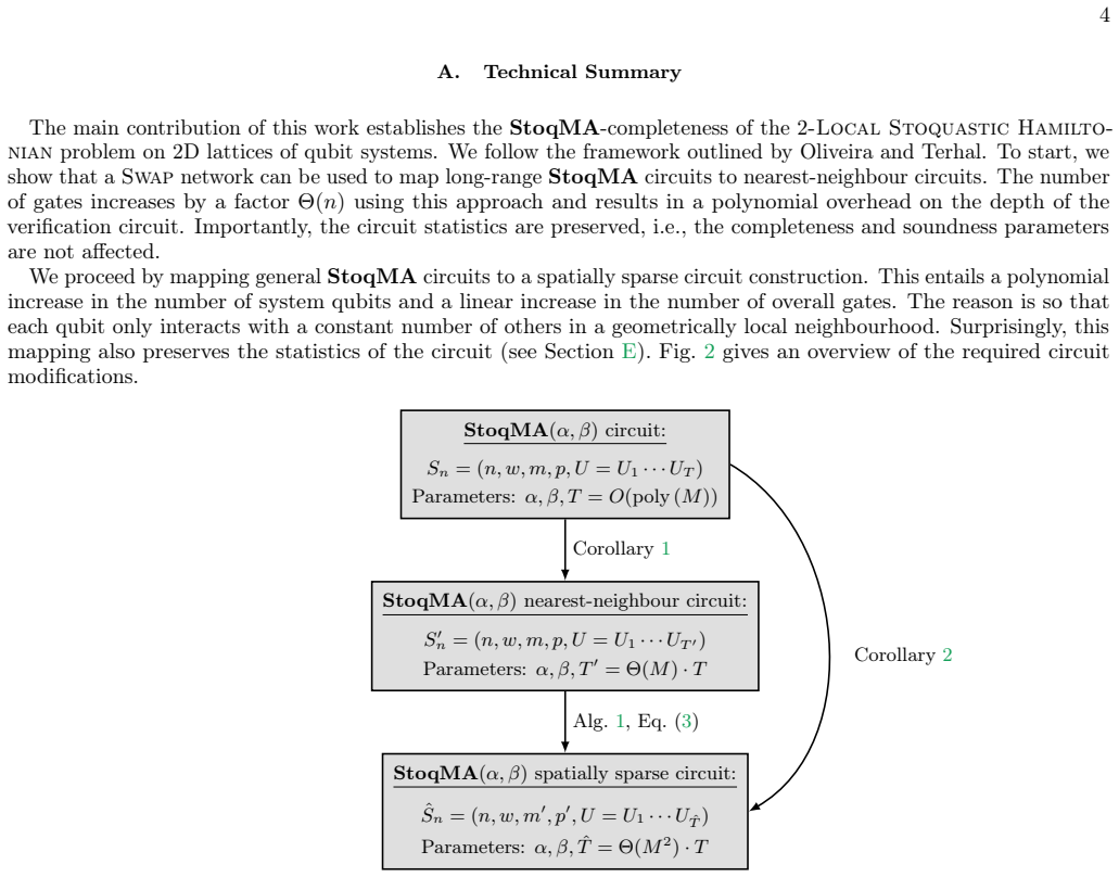
We show the 2-Local Stoquastic Hamiltonian problem on a 2D square qubit lattice is StoqMA-complete. This is achieved by extending the spatially sparse circuit construction and the stoquastic-preserving perturbative gadgets so that StoqMA circuits can be made spatially sparse and geometrical stoquastic-preserving perturbative gadgets can be constructed without an increase to particle dimension.
What carries the argument
Geometrical stoquastic-preserving perturbative gadgets realized on 2D lattices that preserve 2-locality and qubit dimension.
If this is right
- StoqMA-completeness continues to hold when the Hamiltonian is restricted to a 2D square lattice geometry.
- The hardness result requires only 2-local interactions between qubits.
- No increase in the local Hilbert-space dimension is needed to embed the hard instances.
- The spatially sparse StoqMA circuit construction can be embedded directly into the 2D lattice layout.
Where Pith is reading between the lines
- The same geometric gadget constructions could be tested on other regular lattices such as triangular or hexagonal to check whether planarity alone is the key restriction.
- If the gadgets extend to higher dimensions without extra cost, the 2D result would imply that StoqMA-completeness is insensitive to lattice dimension beyond two.
- One could ask whether the same techniques produce hardness for the related problem of sampling from the ground state rather than only approximating its energy.
Load-bearing premise
The extensions of the spatially sparse circuit construction and the stoquastic-preserving perturbative gadgets from prior work can be realized geometrically on a 2D lattice while keeping all interactions 2-local and without increasing the local Hilbert-space dimension.
What would settle it
A classical polynomial-time algorithm that approximates the ground-state energy of every 2-local stoquastic Hamiltonian on a 2D square lattice to inverse-polynomial additive precision would falsify the claim.
Figures





read the original abstract
We show the 2-Local Stoquastic Hamiltonian problem on a 2D square qubit lattice is StoqMA-complete. We achieve this by extending the spatially sparse circuit construction of Oliveira and Terhal, as well as the perturbative gadgets of Bravyi, DiVincenzo, Oliveira, and Terhal. Our main contributions demonstrate StoqMA circuits can be made spatially sparse and that geometrical, stoquastic-preserving, perturbative gadgets can be constructed, without an increase to particle dimension.
Editorial analysis
A structured set of objections, weighed in public.
Referee Report
Summary. The paper claims to prove that the 2-local stoquastic Hamiltonian problem on 2D square qubit lattices is StoqMA-complete. This is done by extending the spatially sparse circuit construction of Oliveira and Terhal together with the stoquastic-preserving perturbative gadgets of Bravyi, DiVincenzo, Oliveira and Terhal so that both constructions can be realized geometrically on a 2D lattice while remaining 2-local, stoquastic, and qubit-dimensional.
Significance. If the central claim holds, the result supplies a natural 2D-lattice StoqMA-complete problem, tightening the complexity landscape for stoquastic Hamiltonians that appear in quantum Monte Carlo and stoquastic quantum simulation. The explicit 2D gadget and sparsity constructions would be reusable tools for future reductions.
major comments (2)
- [Section describing the spatially sparse circuit construction] The geometric embedding of the spatially sparse circuit (main contribution 1) must be shown to preserve 2-locality on the square lattice; any auxiliary long-range couplings introduced by the 2D layout would invalidate the reduction to a valid 2-local StoqMA instance.
- [Section describing the geometrical stoquastic-preserving perturbative gadgets] The stoquastic-preserving perturbative gadgets (main contribution 2) must be shown to cancel all positive off-diagonal matrix elements without either (i) introducing non-2-local terms or (ii) increasing the local Hilbert-space dimension beyond qubits; the manuscript's claim that this is achieved geometrically is load-bearing for the final Hamiltonian remaining a valid StoqMA instance.
Simulated Author's Rebuttal
We thank the referee for their positive evaluation of the significance of our result and for highlighting the key technical requirements for the reduction. We address each major comment below by pointing to the explicit constructions and proofs already present in the manuscript. We believe these sections establish the required properties without introducing invalid terms.
read point-by-point responses
-
Referee: [Section describing the spatially sparse circuit construction] The geometric embedding of the spatially sparse circuit (main contribution 1) must be shown to preserve 2-locality on the square lattice; any auxiliary long-range couplings introduced by the 2D layout would invalidate the reduction to a valid 2-local StoqMA instance.
Authors: The spatially sparse circuit construction is presented in Section 3, where we give an explicit geometric embedding onto the 2D square lattice. The layout routes all circuit wires and gates along nearest-neighbor paths on the grid, using only adjacent qubit interactions; the proof of Theorem 1 explicitly verifies that no auxiliary long-range couplings arise, as crossings and connections are realized through a sequence of 2-local stoquastic terms without non-local jumps. This preserves both 2-locality and the stoquastic property throughout the reduction. revision: no
-
Referee: [Section describing the geometrical stoquastic-preserving perturbative gadgets] The stoquastic-preserving perturbative gadgets (main contribution 2) must be shown to cancel all positive off-diagonal matrix elements without either (i) introducing non-2-local terms or (ii) increasing the local Hilbert-space dimension beyond qubits; the manuscript's claim that this is achieved geometrically is load-bearing for the final Hamiltonian remaining a valid StoqMA instance.
Authors: The geometrical stoquastic-preserving perturbative gadgets are constructed in Section 4. The gadgets are arranged on the 2D lattice such that all mediating interactions are strictly 2-local qubit terms; the perturbative analysis shows that positive off-diagonal elements are exactly canceled in the effective low-energy Hamiltonian while the higher-order terms remain stoquastic and 2-local. The construction uses only qubit degrees of freedom with no increase in local dimension, as stated in the gadget definitions and the effective Hamiltonian derivation following Lemma 2. revision: no
Circularity Check
No circularity: StoqMA-completeness shown via explicit extension of external prior constructions
full rationale
The paper's central claim is a new completeness reduction for 2-local stoquastic Hamiltonians on 2D lattices. It proceeds by extending the spatially sparse circuit construction of Oliveira-Terhal and the perturbative gadgets of Bravyi-DiVincenzo-Oliveira-Terhal to 2D geometry while preserving 2-locality, stoquasticity, and qubit dimension. These source constructions are from independent prior literature; the present work's contribution is the geometric realization on the lattice. No equation reduces a claimed prediction to a fitted parameter, no self-citation chain bears the load, and no ansatz or uniqueness theorem is imported from the authors' own prior work. The derivation is therefore self-contained against external benchmarks.
Axiom & Free-Parameter Ledger
axioms (1)
- standard math Standard definitions and closure properties of the complexity class StoqMA and of stoquastic Hamiltonians as given in prior literature.
Forward citations
Cited by 3 Pith papers
-
The Guided Local Hamiltonian Problem for Stoquastic Hamiltonians
The Guided Local Hamiltonian problem for stoquastic Hamiltonians is promise BPP-hard (even 2-local on lattices), BQP-hard under fixed local constraints, and admits a deterministic classical approximation algorithm whe...
-
Unentangled stoquastic Merlin-Arthur proof systems: the power of unentanglement without destructive interference
StoqMA(2) contains NP with Õ(√n)-qubit proofs and completeness error 2^{-polylog(n)}, is contained in EXP, and satisfies StoqMA(k)=StoqMA(2) for k≥2 when completeness error is negligible.
-
On the Complexity of the Succinct State Local Hamiltonian Problem
The succinct state 2-local Hamiltonian problem for qubit Hamiltonians is promise-MA-complete.
Reference graph
Works this paper leans on
-
[1]
We can now introduce a perturbation gadget to simulate the low-energy spectrum of Eq
It is easy to see C †C and D†D are diagonal. We can now introduce a perturbation gadget to simulate the low-energy spectrum of Eq. (6). Let the target Hamiltonian be Eq. (6) and define the perturbed HamiltonianeH=H+Vwith, H= ∆ MX a=1 |1⟩ ⟨1|a , V= √ ∆V main +V extra, Vmain =− MX a=1 Ca +D † a S+ a + C † a +D a S− a ,(7) Vextra = MX a=1 C † a ⊗C a +D a ⊗D ...
-
[2]
2 S± could be represented as theρ-matricesρ2/ρ1, but we leave them asS± for clarity
Special 3-Local Stoquastic Hamiltonians In order to perform the3-to-2-local reduction of stoquastic Hamiltonians, it is convenient to reduce a general3-local stoquastic Hamiltonian to a special form, H= Γ− X B∈Ω3 hjXj1 Xj2 Xj3 . 2 S± could be represented as theρ-matricesρ2/ρ1, but we leave them asS± for clarity. 16 A general3-local is reduced to the speci...
-
[3]
theSubdivisiongadget,
-
[4]
17 Each gadget serves a specific purpose
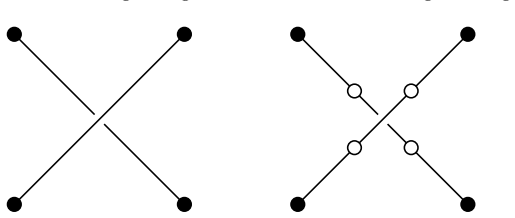
theTrianglegadget. 17 Each gadget serves a specific purpose. TheForkandTrianglegadgets are used to reduce the degree of vertices. TheCrossgadget’s role is to planarise the interaction graph. We have already seen a subdivision gadget. However, we emphasise that a2-local stoquastic interaction can also be subdivided — proving useful for theTriangleand other...
-
[5]
For example, an edge PuPv describes two ρ-matrices acting on vertices u and v and where Pu does not necessarily equalPv. A general interaction edge for these stoquastic Hamiltonians is expressed as PuPv + P † uP † v — this is taken from Eq. (6). For brevity we sayχuv = Pu + P † v and χ† uv = P † u + Pv. Note that the interaction edge PuPv + P † uP † v can...
-
[6]
each vertexu∈ V(G)is mapped to a lattice siteϕ(u)∈ V(Λ)within the boundary ∂Λ = [−O(|V(G)|), O(|V(G)|)] 2,
-
[7]
TheSubdivisiongadget can be used to map the edges{u, v} to lattice pathsϕ({u, v})
each edge {u, v} ∈ E (G)is mapped to a lattice pathϕ({u, v}) ∈ E (Λ)of length O(1)between ϕ(u)and ϕ(v) without crossing any other lattice path. TheSubdivisiongadget can be used to map the edges{u, v} to lattice pathsϕ({u, v}). We must ensure that the lattice paths remain close to the original edges they are associated with. For a sufficiently fine grid, t...
-
[8]
A. Y. Kitaev, A. H. Shen, and M. N. Vyalyi,Classical and Quantum Computation(American Mathematical Society, USA, 2002)
work page 2002
-
[9]
R. Oliveira and B. M. Terhal, Quantum Info. Comput.8, 900 (2008), arXiv:0504050
work page 2008
-
[10]
N. Schuch and F. Verstraete, Nature Physics5, 732 (2009), arXiv:0712.0483
work page internal anchor Pith review Pith/arXiv arXiv 2009
-
[11]
The complexity of antiferromagnetic interactions and 2D lattices
S. Piddock and A. Montanaro, Quantum Info. Comput.17, 636 (2017), arXiv:1506.04014
work page internal anchor Pith review Pith/arXiv arXiv 2017
-
[12]
T. S. Cubitt and A. Montanaro, inProceedings of the 2014 IEEE 55th Annual Symposium on Foundations of Computer Science, FOCS ’14 (IEEE Computer Society, USA, 2014) pp. 120–129, arXiv:1311.3161
work page internal anchor Pith review Pith/arXiv arXiv 2014
- [13]
- [14]
-
[15]
J. D. Biamonte and P. J. Love, Physical Review A78, 10.1103/physreva.78.012352 (2008), arXiv:0704.1287
work page internal anchor Pith review Pith/arXiv arXiv doi:10.1103/physreva.78.012352 2008
-
[16]
S. Bravyi and M. Vyalyi, Quantum Info. Comput.5, 187 (2005), arXiv:0308021
work page 2005
-
[17]
Complexity of commuting Hamiltonians on a square lattice of qubits
N. Schuch, Quantum Info. Comput.11, 901 (2011), arXiv:1105.2843
work page internal anchor Pith review Pith/arXiv arXiv 2011
-
[18]
D. Aharonov and L. Eldar, inProceedings of the 2011 IEEE 52nd Annual Symposium on Foundations of Computer Science, FOCS ’11 (IEEE Computer Society, USA, 2011) pp. 334–343, arXiv:1102.0770
work page internal anchor Pith review Pith/arXiv arXiv 2011
-
[19]
The commuting local Hamiltonian on locally-expanding graphs is in NP
D. Aharonov and L. Eldar, Quantum Information Processing14, 83 (2014), arXiv:1311.7378
work page internal anchor Pith review Pith/arXiv arXiv 2014
-
[20]
D. Aharonov, O. Kenneth, and I. Vigdorovich, in13th Conference on the Theory of Quantum Computation, Communi- cation and Cryptography (TQC 2018), Vol. 111 (Schloss Dagstuhl – Leibniz-Zentrum für Informatik, 2018) pp. 2:1–2:21, arXiv:1803.02213
-
[21]
S. Irani and J. Jiang, Commuting local Hamiltonian problem on 2D beyond qubits (2023), arXiv:2309.04910
-
[22]
E. Y. Loh, J. E. Gubernatis, R. T. Scalettar, S. R. White, D. J. Scalapino, and R. L. Sugar, Phys. Rev. B41, 9301 (1990)
work page 1990
-
[23]
Sign-Problem-Free Fermionic Quantum Monte Carlo: Developments and Applications
Z.-X. Li and H. Yao, Annual Review of Condensed Matter Physics10, 337 (2019), arXiv:1805.08219
work page internal anchor Pith review Pith/arXiv arXiv 2019
-
[24]
D. Hangleiter, I. Roth, D. Nagaj, and J. Eisert, Science Advances6, 10.1126/sciadv.abb8341 (2020), arXiv:1906.02309
-
[25]
W. M. C. Foulkes, L. Mitas, R. J. Needs, and G. Rajagopal, Rev. Mod. Phys.73, 33 (2001)
work page 2001
-
[26]
A. W. Sandvik, A. Avella, and F. Mancini, inAIP Conference Proceedings(AIP, 2010) arXiv:1101.3281
work page internal anchor Pith review Pith/arXiv arXiv 2010
-
[27]
M. Ohzeki, Scientific Reports7, 10.1038/srep41186 (2017), arXiv:1612.04785
work page internal anchor Pith review Pith/arXiv arXiv doi:10.1038/srep41186 2017
- [28]
- [29]
-
[30]
D. F. B. ten Haaf, H. J. M. van Bemmel, J. M. J. van Leeuwen, W. van Saarloos, and D. M. Ceperley, Phys. Rev. B51, 13039 (1995)
work page 1995
-
[31]
D. Aharonov, A. B. Grilo, and Y. Liu, StoqMA vs. MA: the power of error reduction (2021), arXiv:2010.02835 [quant-ph]
-
[32]
Y. Liu, in16th Conference on the Theory of Quantum Computation, Communication and Cryptography (TQC 2021), Vol. 197 (Schloss Dagstuhl – Leibniz-Zentrum für Informatik, 2021) pp. 4:1–4:22, arXiv:2011.05733
-
[33]
C. Marriott and J. Watrous, Computational Complexity14, 122 (2005), arXiv:0506068
work page 2005
-
[34]
Complexity of stoquastic frustration-free Hamiltonians
S. Bravyi and B. Terhal, SIAM J. Comput.39, 1462 (2009), arXiv:0806.1746
work page internal anchor Pith review Pith/arXiv arXiv 2009
-
[35]
On complexity of the quantum Ising model
S. Bravyi and M. Hastings, Communications in Mathematical Physics349, 1 (2016), arXiv:1410.0703
work page internal anchor Pith review Pith/arXiv arXiv 2016
- [36]
- [37]
-
[38]
Gharibian, SIGACT News54, 54 (2024), arXiv:2310.18010
S. Gharibian, SIGACT News54, 54 (2024), arXiv:2310.18010
-
[39]
S. Zachos and M. Furer, inProc. of the Seventh Conference on Foundations of Software Technology and Theoretical Computer Science(Springer-Verlag, Berlin, Heidelberg, 1987) pp. 443–455
work page 1987
- [40]
-
[41]
Schrieffer-Wolff transformation for quantum many-body systems
S. Bravyi, D. P. DiVincenzo, and D. Loss, Annals of Physics326, 2793 (2011), arXiv:1105.0675. 27
work page internal anchor Pith review Pith/arXiv arXiv 2011
-
[42]
Simulation of Many-Body Hamiltonians using Perturbation Theory with Bounded-Strength Interactions
S. Bravyi, D. P. DiVincenzo, D. Loss, and B. M. Terhal, Phys. Rev. Lett.101, 070503 (2008), arXiv:0803.2686
work page internal anchor Pith review Pith/arXiv arXiv 2008
- [43]
-
[44]
A. L. Fetter, J. D. Walecka, and L. P. Kadanoff,Quantum theory of many-particle sys, Dover Books on Physics (Dover Publications, Mineola, NY, 2003)
work page 2003
-
[45]
M. Ioannou, S. Piddock, M. Marvian, J. Klassen, and B. M. Terhal, Termwise versus globally stoquastic local Hamiltonians: questions of complexity and sign-curing (2022), arXiv:2007.11964
-
[46]
Polynomial-time classical simulation of quantum ferromagnets
S. Bravyi and D. Gosset, Phys. Rev. Lett.119, 100503 (2017), arXiv:1612.05602
work page internal anchor Pith review Pith/arXiv arXiv 2017
-
[47]
S. Piddock,Complexity and Simulation of Many-Body Quantum Systems, Phd thesis, University of Bristol (2019)
work page 2019
-
[48]
Monte Carlo simulation of stoquastic Hamiltonians
S. Bravyi, Quantum Info. Comput.15, 1122 (2015), arXiv:1402.2295
work page internal anchor Pith review Pith/arXiv arXiv 2015
-
[49]
A. B. Grilo, I. Kerenidis, and J. Sikora, Qma with subset state witnesses, inMathematical Foundations of Computer Science 2015(Springer Berlin Heidelberg, 2015) pp. 163–174, arXiv:1410.2882
work page internal anchor Pith review Pith/arXiv arXiv 2015
-
[50]
S. Gharibian and F. Le Gall, SIAM Journal on Computing52, 1009 (2023), arXiv:2111.09079. Appendix A: Parallel Gadget Application When employing perturbation gadgets, it is important to ensure they do not cross-interfere and create unwanted interaction terms. For each gadget considered in this work, no construction, to the appropriate order, suffers any un...
-
[51]
Subdivision and Geometrical Gadgets The subdivision gadget and all geometrical gadgets,Subdivision,CrossandFork, use the same unperturbed penalty Hamiltonian. For a series of edges that are acted upon by these perturbation gadgets in parallel, we must show that there are no cross-gadget terms to second-order. The unperturbed penalty Hamiltonian is given b...
-
[52]
We must show that to second-order there are no cross-gadget terms
3-to-2-Local Gadgets When reducing a3-local stoquastic Hamiltonian to a2-local one, the specific gadget is used in parallel across all interaction edges inΩ 3. We must show that to second-order there are no cross-gadget terms. This perturbation technique uses a third-order construction. The first-order and second-order corrections simply create energy shi...
-
[53]
The calculation of the effective Hamiltonian is similar to Section A1, thus using Lemma 2 we have that Heff. = MX a=1 C † aCa +D aD† a − − X a,b,c √ ∆ Ca +D † a S+ a + C † a +D a S− a −+ × 1 ∆ |1⟩ ⟨1|b √ ∆ Cc +D † c S+ c + C † c +D c S− c +− . The key terms to analyse are(S± a )−+ |1⟩ ⟨1|b (S± c )+−. Trivially,(S + a )−+ = 0and(S − a )+− = 0. It is not ha...
- [54]
-
[55]
010. . .0 , where the1is in the a-th position. The only terms that survive in the latter half of the above expression are thus given by S− a −+ |1⟩ ⟨1|b S+ c +− =δ abδbc 0M 0M , reducing the overall effective Hamiltonian to Heff. = MX a=1 C † aCa +D aD† a 0M 0M − MX a=1 Ca +D † a C † a +D a 0M 0M , Heff. =− MX a=1 CaDa +D † aC † a 0M 0M . This concludes t...
discussion (0)
Sign in with ORCID, Apple, or X to comment. Anyone can read and Pith papers without signing in.