REVIEW 3 major objections 8 minor 43 references
Decoding Latent Spaces: Assessing the Interpretability of Time Series Foundation Models for Visual Analytics
T0 review · 3 major / 8 minor · reviewed 2026-08-16 · deepseek-v4-flash
Pith's one-line read Fine-tuning a time-series foundation model lowers reconstruction loss, but its latent-space projections stay just as hard to read.
desk verdict A useful, honest negative result: fine-tuning MOMENT reduces reconstruction loss but doesn't visibly improve its embedding projections, though the evidence is only visual. read the letter →
The pith
A machine-rendered reading of the paper's core claim, the machinery that carries it, and where it could break.
The reading
What carries the argument
The mechanism that carries the argument is the pairing of MOMENT's patch-based transformer embeddings with a fixed visual-analysis protocol: time series are cut into windows, embedded by the model, then projected to two dimensions with UMAP followed by PCA for inspection in DeepVATS. The comparison of loss improvement, defined as the percent reduction in masked mean-squared error before versus after fine-tuning, against the visual structure of these projections is what allows the paper to separate quantitative adaptation from interpretability. Fine-tuning itself is done as a masked-imputation task with four tunable parameters: the percentage of data used for training, the validation percentage, the mask percentage, and the number of Fourier-selected window lengths.
What would settle it
Compute cluster-separation metrics, such as silhouette score or cluster purity, on the raw embeddings before any projection for zero-shot versus fine-tuned MOMENT models on the S1 segmentation dataset; if these metrics improve substantially after fine-tuning, the claim that loss gains do not translate into embedding precision would need to be revised.
Extended reading notes
Core claim
The central claim is that for the MOMENT family of multivariate time-series foundation models, reductions in reconstruction loss after task-specific fine-tuning do not translate into clearer latent-space projections. Across segmentation, anomaly-detection, and trend datasets (S1, S2, S3, M-Toy, and Kohl's), both zero-shot and fine-tuned versions produced embedding plots with interlinked clusters; the same segments, anomalies, and trends were equally hard to isolate before and after training. MOMENT-small showed the largest loss improvements (around 22 percent), MOMENT-base the clearest partial segmentation of the S1 series, and MOMENT-large the most defined clusters for anomaly detection, yet no model version showed a visually interpretable separation of trends, and fine-tuning rarely changed the projection beyond rotations or subtle rearrangements. The paper therefore argues that the apparent understanding gained by the model, as measured by loss, is not reflected in projection-based interpretability, and that the MOMENT embeddings may need alternative projection methods, loss functions, or preprocessing to support visual analytics.
Load-bearing premise
The negative conclusion assumes that the UMAP-then-PCA projections used in the DeepVATS pipeline faithfully expose the structure of the high-dimensional embeddings; if a different projection would reveal clear clusters, the visual result would be an artifact of the projection rather than of the embeddings.
Editorial extensions
If this is right
- Reconstruction loss should not be used as a proxy for embedding clarity in visual-analytics applications; a model can appear to improve numerically while its projected clusters stay just as tangled.
- For interactive visual analytics, the smallest model version is the most attractive: it had the largest loss reduction, similar interpretability to the larger versions, and lower computation and memory cost.
- Fine-tuning with a small fraction of the data (15 to 20 percent) and a modest number of epochs is enough to change model behavior, so heavy training is not required for adaptation.
- Time-series foundation models can replace task-specific autoencoders in visual-analytics pipelines, cutting waiting time while retaining pattern detection, but they do not yet provide clear segment and trend structure by default.
- Improving interpretability will require modifying the pipeline itself, for example by trying alternative projection techniques, loss functions such as soft-DTW, or data preprocessing, rather than simply fine-tuning longer.
Reading between the lines
- Going beyond the paper, the negative visual result may be an artifact of the projection: UMAP followed by PCA with fixed parameters can obscure structure that a different projection, such as t-SNE or PacMAP, might reveal.
- A natural testable extension is to measure cluster purity or silhouette scores on the raw embeddings before projection; if those metrics improve after fine-tuning while the projected plots do not, the bottleneck is visualization, not the model's internal geometry.
- If the projection-artifact explanation holds, the same experimental design could serve as a reusable benchmark for future time-series foundation models, provided that projection-free interpretability metrics are added alongside the visual inspection.
Signed reviews
Editorial analysis
A structured set of objections, weighed in public.
Referee Report
Summary. This paper integrates the MOMENT family of time series foundation models into the DeepVATS visual analytics framework and studies whether zero-shot and fine-tuned MOMENT embeddings yield visually interpretable projections for segmentation, anomaly, pattern, and trend detection. The authors evaluate MOMENT-small/base/large on five datasets (S1, S2, S3, M-Toy, Kohl's), fine-tune the models with a masked-reconstruction objective, select hyperparameters via feature-importance analysis on Kohl's, and compare loss improvements with visual inspection of UMAP-then-PCA scatter plots. They report substantial loss reductions after fine-tuning (up to ~22%) but little visible improvement in embedding interpretability, and conclude that quantitative improvements are not necessarily linked to embedding precision. The paper's stated contribution is the first integration of a foundation model into a visual analytics tool, with a wrapper for fine-tuning arbitrary torch-based models.
Significance. If the negative visual result were backed by quantitative evidence, the paper would be a useful cautionary case study for the visual analytics and time-series foundation model communities: it would show that reconstruction-loss gains do not automatically translate into human-interpretable projections and would motivate alternative projection/loss/preprocessing choices. The paper has concrete strengths: code is promised via a GitHub footnote, the study covers three model sizes and five datasets, the statistical analysis uses multiple feature-importance estimators (SelectKBest, Random Forest, SHAP, and correlation), and the integration wrapper is a reusable engineering contribution. However, the central conclusion rests on the authors' subjective reading of scatter plots; no quantitative interpretability metric, no inter-rater reliability, no ablation of projection choice, and no repeated-run variance are reported. Because the projection pipeline (UMAP followed by PCA) is inherited from the earlier MTSAE-based DeepVATS study and not validated for MOMENT embeddings, the stress-test concern lands: the negative finding is currently indistinguishable from a projection artifact.
major comments (3)
- [§III.D–IV, Figs. 10–22] The central claim that fine-tuning does not improve embedding interpretability is based solely on the authors' visual comparison of scatter plots. No quantitative interpretability metric (e.g., cluster purity, silhouette score, label-aware separation, or projection trustworthiness) is computed on the raw MOMENT embeddings; no inter-rater reliability is reported; and UMAP stochasticity is not controlled by repeated runs or fixed seeds. The paper's own Section IV recommends testing alternative projection methods (e.g., PCA without UMAP and t-SNE), which concedes that the current projection may obscure genuine structure. To make the negative visual result load-bearing, the authors should report embedding-space quality metrics computed before projection, repeat UMAP with several seeds, and compare at least one alternative projection method. Without this, the conclusion that fine-tuning leaves the embeddings visually unchanged is not distinguishable from a projection artifact.
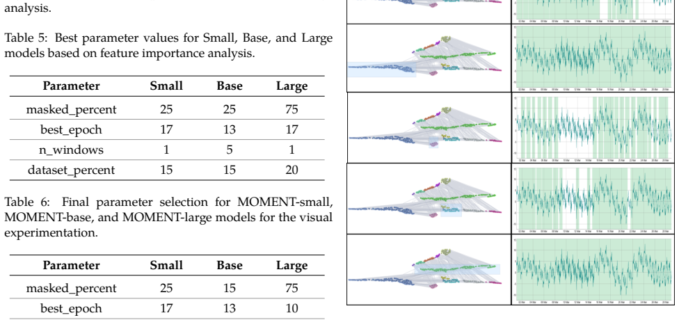
- [§III.C, Tables 5–6] The hyperparameter selection procedure is not sufficiently justified or robust. The grid is first reduced from 72 to 18 cases for computational reasons, and the final parameters in Table 6 differ from the 'best' values in Table 5 (e.g., MOMENT-base masked_percent changes from 25 to 15 and dataset_percent from 15 to 25; MOMENT-large best_epoch changes from 17 to 10) without explanation of the cost-to-improvement trade-off used. These hyperparameters are tuned on the Kohl's time series and then applied to all other datasets (S1, S2, S3, M-Toy), yet no justification is given for transferring them across datasets with different structure. In addition, the reported loss improvements are single-run values without standard errors or repeated seeds, so the 22% / 10% / 4% improvements cannot be assessed for stability. The authors should report variance across runs and justify the final parameter choices, or the fine-tuning comparison is not reliably interpretable.
- [§III.C–IV, RQ1] The paper conflates reconstruction loss with embedding geometry. The improvement metric is the masked reconstruction loss improvement, defined as (loss_first − loss_final)/loss_first × 100 in §III.C. No measure of how much the embedding vectors themselves changed (e.g., mean cosine or euclidean displacement, nearest-neighbor overlap) is reported, and the phrase 'embeddings precision' in the Introduction and Conclusions is never defined. Consequently, the conclusion that 'quantitative improvements are not necessarily linked to the embeddings precision' is not supported by the measurements presented; a visually unchanged projection could reflect unchanged embeddings, projection insensitivity, or dominant seed and hyperparameter variation. The authors should either define and measure embedding-space change directly or soften the claim to refer specifically to reconstruction loss.
minor comments (8)
- [Throughout] The manuscript needs thorough language editing; there are numerous typos and grammatical errors (e.g., 'supose', 'wether', 'apportation', 'intrinsecal', 'diferent', 'descripted', 'freexing', 'difficultying').
- [Appendix B.1, Figs. 40–42] The caption text says these figures show 'MOMENT-small for S1', but Section III.E and the surrounding analysis refer to MOMENT-base clusters; the caption should be corrected to MOMENT-base.
- [Appendix A, Figs. 29–31] The captions labeled 'From top to botton, the linear correlation matrices for MOMENT-small/base/large' do not match the surrounding text, which describes these figures as the frequency of the best epoch; the captions should be corrected.
- [Table 4] The column header 'Best %' in Table 4 is inconsistent with the 'KBest %' header used in Tables 2 and 3; the table also should state how the percentages are normalized across the four feature-importance estimators.
- [Tables 11–12] The summary table is numbered Table 12 although no Table 11 appears in the text; renumber the tables sequentially.
- [§III.C] The text says the full grid has 72 cases and then reduces it to 18 cases due to computational cost; please state exactly which of the 72 configurations were actually run and whether the reduction was a random subsample or a systematic restriction.
- [§IV] The claim that foundation models 'supose a big reduction in execution time' is not supported by any runtime measurements in the paper; if kept, it should be backed by measured training or inference times or removed.
- [§I] The claim of being 'the first integration of foundation models into visual analytics tools' is stated without a systematic comparison to existing work; please soften the novelty claim or provide evidence from a broader literature search.
Circularity Check
No significant circularity: the negative visual finding is empirical and not forced by the loss objective; self-citations to DeepVATS are methodological context, not load-bearing.
full rationale
The paper's central claim is that fine-tuning MOMENT reduces masked reconstruction loss but does not produce visually more interpretable UMAP-then-PCA embedding projections. This is an empirical conjunction of two measurements, not a derivation. The loss improvement is computed from the fine-tuning objective as (loss_first - loss_final) * 100 / loss_first, while interpretability is assessed qualitatively from scatter plots in Figures 10-22 and summarized in Tables 7-10. Neither quantity is defined in terms of the other, and no equation in the paper forces the visual outcome to follow from the loss reduction. Hyperparameters are selected on Kohl's loss in Section III.C, but the visual comparison is performed on fine-tuned models across S1-S3, M-Toy, and Kohl's; the visual result is not a function of the fitted loss objective. The only notable self-citations are the use of DeepVATS [5] as the evaluation framework and as the source of datasets and projection choices, plus prior MPlot work [13]-[14]; these are methodological inheritance rather than load-bearing premises, and the paper's negative visual finding is exhibited directly in the figures rather than imported from those citations. Concerns that the inherited projection may hide structure are a validity threat, and the paper itself suggests testing alternative projection methods in Section IV, but this does not amount to a circular reduction. No uniqueness theorem, no ansatz smuggled in via citation, and no renaming of a known result was found.
Assumptions & free parameters
free parameters (6)
- masked_percent =
Small: 25, Base: 15, Large: 75
- best_epoch =
Small: 17, Base: 13, Large: 10 (final selection)
- n_windows =
Small: 1, Base: 5, Large: 1
- dataset_percent =
Small: 15, Base: 25, Large: 20
- window_lengths =
17 plus Fourier-selected dominant sizes (find_dominant_window_sizes from aeon)
- Projection hyperparameters for UMAP and PCA =
Not specified (defaults or inherited from DeepVATS)
assumptions (5)
- domain assumption MOMENT's pretrained embedding outputs are appropriate inputs for visual analysis of time series structure.
- domain assumption Masked reconstruction (imputation) loss is a meaningful fine-tuning objective for improving embedding quality.
- domain assumption UMAP followed by PCA projections reveal the structure relevant to human interpretation.
- domain assumption Reference labels and definitions for segments, anomalies, and trends in S1-S3, M-Toy, and Kohl's are correct.
- standard math Underlying software libraries (PyTorch, tsai, aeon) behave as documented.
Cite this review
Pith. "Pith review of Decoding Latent Spaces: Assessing the Interpretability of Time Series Foundation Models for Visual Analytics." pith.science (2026). https://pith.science/paper/QDLDZE5F
@misc{pith2026250420099,
  author       = {Pith},
  title        = {Pith review of: Decoding Latent Spaces: Assessing the Interpretability of Time Series Foundation Models for Visual Analytics},
  year         = {2026},
  howpublished = {\url{https://pith.science/paper/QDLDZE5F}},
  note         = {Machine review of arXiv:2504.20099}
}
read the original abstract
The present study explores the interpretability of latent spaces produced by time series foundation models, focusing on their potential for visual analysis tasks. Specifically, we evaluate the MOMENT family of models, a set of transformer-based, pre-trained architectures for multivariate time series tasks such as: imputation, prediction, classification, and anomaly detection. We evaluate the capacity of these models on five datasets to capture the underlying structures in time series data within their latent space projection and validate whether fine tuning improves the clarity of the resulting embedding spaces. Notable performance improvements in terms of loss reduction were observed after fine tuning. Visual analysis shows limited improvement in the interpretability of the embeddings, requiring further work. Results suggest that, although Time Series Foundation Models such as MOMENT are robust, their latent spaces may require additional methodological refinements to be adequately interpreted, such as alternative projection techniques, loss functions, or data preprocessing strategies. Despite the limitations of MOMENT, foundation models supose a big reduction in execution time and so a great advance for interactive visual analytics.
Figures


Figures from the paper (42 more)




Reference graph
Works this paper leans on
-
[1]
From requirement to solution: Unveiling problem-driven design patterns in visual analytics,
Y.Wu,S.Gao,S.Zhang,X.Dou,X.Wang,Q.Li,“From requirement to solution: Unveiling problem-driven design patterns in visual analytics,”IEEE Transactions on Visualization and Computer Graphics, 2025
work page 2025
-
[2]
Visual causal analysis of multivariate time series,
X. Zhang, X. Yang, H. Hu, H. Qin, “Visual causal analysis of multivariate time series,” Journal of Visualization, pp. 1–17, 2025
work page 2025
-
[3]
Embedding projector - visualization of high-dimensional data,
TensorFlow, “Embedding projector - visualization of high-dimensional data,” 08 2023. [Online]. Available: https://projector.tensorflow.org/, Accessed: 2024-07- 02
work page 2023
- [4]
-
[5]
Deepvats: Deep visual analytics for time series,
V. Rodriguez-Fernandez, D. Montalvo-Garcia, F. Piccialli, G. J. Nalepa, D. Camacho, “Deepvats: Deep visual analytics for time series,” Knowledge- Based Systems , vol. 277, p. 110793, 2023, doi: 10.1016/j.knosys.2023.110793
arXiv 2023
-
[6]
Pushing the limits of pre-training for time series forecasting in thecloudopsdomain,
G. Woo, C. Liu, A. Kumar, D. Sahoo, “Pushing the limits of pre-training for time series forecasting in thecloudopsdomain,” arXivpreprintarXiv:2310.05063 , 2023
arXiv 2023
-
[7]
Mixed contrastive transfer learning for few-shot workload predictioninthecloud,
Z. Zuo, Y. Huang, Z. Li, Y. Jiang, C. Liu, “Mixed contrastive transfer learning for few-shot workload predictioninthecloud,” Computing,vol.107,no.1,p.5, 2025
work page 2025
-
[8]
A. G. Meyer, F. Lu, L. Clemente, M. Santillana, “A prospective real-time transfer learning approach to estimate influenza hospitalizations with limited data,” Epidemics, p. 100816, 2025
work page 2025
Show all 43 references
-
[9]
Transfer learning for time series classification,
H. I. Fawaz, G. Forestier, J. Weber, L. Idoumghar, P.-A. Muller, “Transfer learning for time series classification,” in2018 IEEE international conference on big data (Big Data), 2018, pp. 1367–1376, IEEE
2018
- [10]
-
[11]
Chronos: Learning the language of time series,
A. F. Ansari, L. Stella, C. Turkmen, X. Zhang, P. Mercado, H. Shen, O. Shchur, S. Rangapuram, S. P. Arango, S. Kapoor, J. Zschiegner, D. M. Robinson, H. Wang, M. Mahoney, K. Torkkola, A. Wilson, M. Bohlke-Schneider, Y. B. Wang, “Chronos: Learning the language of time series,”T...
2024
-
[12]
Unified training of universal time series forecastingtransformers,
G. Woo, C. Liu, A. Kumar, C. Xiong, S. Savarese, D. Sahoo, “Unified training of universal time series forecastingtransformers,”in 41InternationalConference on Machine Learning (ICML 2024), 2024, pp. 38–44, PMLR
2024
-
[13]
On the integration of large-scale time series distance matrices into deep visual analytic tools,
I. Santamaria-Valenzuela, V. Rodriguez-Fernandez, D. Camacho, “On the integration of large-scale time series distance matrices into deep visual analytic tools,”Cognitive Computation, vol. 17, no. 29, 2025, doi: 10.1007/s12559-024-10394-x
2025 doi
-
[14]
Exploring scalability in large-scale time seriesindeepvatsframework,
I. Santamaria-Valenzuela, V. Rodriguez-Fernandez, D. Camacho, “Exploring scalability in large-scale time seriesindeepvatsframework,”in The13thConferenceon Information Technology and its Applications, Cham, 2024, pp. 244–255, Vietnam - Korea University, Springer Nature Switzerland
2024
-
[15]
Introducing mplots: scaling time series recurrence plots to massive datasets,
M. Shahcheraghi, R. Mercer, J. M. d. A. Rodrigues, A. Der, H. F. S. Gamboa, Z. Zimmerman, K. Mauck, E. Keogh, “Introducing mplots: scaling time series recurrence plots to massive datasets,”Journal of Big Data, vol. 11, no. 1, p. 96, 2024, doi: 10.1186/s40537- 024-00954-1. 20
2024 doi
-
[16]
A systematic review for transformer-based long-term series forecasting,
L. Su, X. Zuo, R. Li, X. Wang, H. Zhao, B. Huang, “A systematic review for transformer-based long-term series forecasting,”Artificial Intelligence Review, vol. 58, no. 3, p. 80, 2025
2025
-
[17]
Are transformers effective for time series forecasting?,
A. Zeng, M. Chen, L. Zhang, Q. Xu, “Are transformers effective for time series forecasting?,” inProceedings of theAAAIconferenceonartificialintelligence ,vol.37,2023, pp. 11121–11128
2023
-
[18]
Autoformer: Decomposition transformers with auto-correlation for long-term series forecasting,
H. Wu, J. Xu, J. Wang, M. Long, “Autoformer: Decomposition transformers with auto-correlation for long-term series forecasting,” Advances in neural information processing systems, vol. 34, pp. 22419–22430, 2021
2021
-
[19]
Attention is all you need,
A. Vaswani, N. Shazeer, N. Parmar, J. Uszkoreit, L. Jones, A. N. Gomez, Ł. Kaiser, I. Polosukhin, “Attention is all you need,” Advances in neural information processing systems, vol. 30, 2017
2017
-
[20]
Timexer: Empowering transformers for time series forecasting with exogenous variables,
Y. Wang, H. Wu, J. Dong, G. Qin, H. Zhang, Y. Liu, Y. Qiu, J. Wang, M. Long, “Timexer: Empowering transformers for time series forecasting with exogenous variables,” Advances in Neural Information Processing Systems, vol. 37, pp. 469–498, 2025
2025
-
[21]
Medformer: A multi-granularity patching transformer for medical time-series classification,
Y. Wang, N. Huang, T. Li, Y. Yan, X. Zhang, “Medformer: A multi-granularity patching transformer for medical time-series classification,” Advances in Neural Information Processing Systems , vol. 37, pp. 36314–36341, 2025
2025
-
[22]
Transfer learning in sensor- based human activity recognition: A survey,
S. G. Dhekane, T. Ploetz, “Transfer learning in sensor- based human activity recognition: A survey,” ACM Computing Surveys, 2025
2025
-
[23]
Foundation models defining a new era in vision: a survey and outlook,
M. Awais, M. Naseer, S. Khan, R. M. Anwer, H. Cholakkal, M. Shah, M.-H. Yang, F. S. Khan, “Foundation models defining a new era in vision: a survey and outlook,” IEEE Transactions on Pattern Analysis and Machine Intelligence, 2025
2025
-
[24]
Advancing domain-specific adaptationsoflargelanguagemodelsthroughtransfer learning and fine-tuning techniques: An analytical study,
A. Rupa, C. Swapna, “Advancing domain-specific adaptationsoflargelanguagemodelsthroughtransfer learning and fine-tuning techniques: An analytical study,”Sentiment Analysis Unveiled, pp. 58–73, 2025
2025
-
[25]
Recentadvancesoffoundationlanguage models-based continual learning: A survey,
Y. Yang, J. Zhou, X. Ding, T. Huai, S. Liu, Q. Chen, Y.Xie,L.He,“Recentadvancesoffoundationlanguage models-based continual learning: A survey,” ACM Computing Surveys, vol. 57, no. 5, pp. 1–38, 2025
2025
-
[26]
Data foundations for large scale multimodal clinical foundation models,
W.Dai,P.Chen,M.Lu,D.Li,H.Wei,H.Cui,P.P.Liang, “Data foundations for large scale multimodal clinical foundation models,” arXiv preprint arXiv:2503.07667, 2025
2025 arXiv
-
[27]
Timegpt-1,
A. Garza, C. Challu, M. Mergenthaler-Canseco, “Timegpt-1,”arXiv preprint arXiv:2310.03589, 2023
2023 arXiv
-
[28]
Lag-llama: Towards foundation models for time series forecasting,
K. Rasul, A. Ashok, A. R. Williams, A. Khorasani, G. Adamopoulos, R. Bhagwatkar, M. Biloš, H. Ghonia, N. Hassen, A. Schneider,et al., “Lag-llama: Towards foundation models for time series forecasting,” inR0- FoMo: Robustness of Few-shot and Zero-shot Learning in Large Foundati...
2023
-
[29]
Visualizing data using t-sne.,
L. Van der Maaten, G. Hinton, “Visualizing data using t-sne.,”Journalofmachinelearningresearch ,vol.9,no.11, 2008
2008
- [30]
-
[31]
Understanding how dimension reduction tools work: An empirical approach to deciphering t-sne, umap, trimap, and pacmap for data visualization,
Y. Wang, H. Huang, C. Rudin, Y. Shaposhnik, “Understanding how dimension reduction tools work: An empirical approach to deciphering t-sne, umap, trimap, and pacmap for data visualization,”Journal of Machine Learning Research, vol. 22, no. 201, pp. 1–73, 2021
2021
-
[32]
Combining dataminingandvisualization: Umaponrope,
S. Bhatnagar, A. Singh, V. Awasthi, S. SK, “Combining dataminingandvisualization: Umaponrope,”in 2024 International Conference on IoT Based Control Networks and Intelligent Systems (ICICNIS), 2024, pp. 1623–1629, IEEE
2024
-
[33]
Dafted: Decoupled asymmetric fusion of tabular and echocardiographic data for cardiac hypertension diagnosis,
J. Stym-Popper, N. Painchaud, P.-Y. COURAND, C. Rambour, N. Thome, O. Bernard, “Dafted: Decoupled asymmetric fusion of tabular and echocardiographic data for cardiac hypertension diagnosis,” in Medical Imaging with Deep Learning , 2025
2025
-
[34]
Timecluster: dimension reduction applied to temporal data for visual analytics,
M. Ali, M. W. Jones, X. Xie, M. Williams, “Timecluster: dimension reduction applied to temporal data for visual analytics,”The Visual Computer, vol. 35, no. 6-8, pp. 1013–1026, 2019
2019
-
[35]
Human-in-the-loop: visual analytics for building models recognising behavioural patterns in time series,
N. Andrienko, G. Andrienko, A. Artikis, P. Mantenoglou, S. Rinzivillo, “Human-in-the-loop: visual analytics for building models recognising behavioural patterns in time series,” IEEE Computer Graphics and Applications, 2024
2024
-
[36]
tsai - a state-of-the-art deep learning library for time series and sequential data
I. Oguiza, “tsai - a state-of-the-art deep learning library for time series and sequential data.” Github, 2023. [Online]. Available: https://github.com/timeseriesAI/tsai
2023
-
[37]
Inceptiontime: Findingalexnetfor time series classification,
H. Ismail Fawaz, B. Lucas, G. Forestier, C. Pelletier, D.F.Schmidt,J.Weber,G.I.Webb,L.Idoumghar,P.-A. Muller,F.Petitjean,“Inceptiontime: Findingalexnetfor time series classification,”Data Mining and Knowledge Discovery, vol. 34, no. 6, pp. 1936–1962, 2020
1936
-
[38]
STUMPY:APowerfulandScalablePython Library for Time Series Data Mining,
S.M.Law, “STUMPY:APowerfulandScalablePython Library for Time Series Data Mining,”The Journal of Open Source Software, vol. 4, no. 39, p. 1504, 2019, doi: 10.21105/joss.01504
2019 doi
-
[39]
The web as a jungle: Non-linear dynamical systems for co-evolving online activities,
Y. Matsubara, Y. Sakurai, C. Faloutsos, “The web as a jungle: Non-linear dynamical systems for co-evolving online activities,” inProceedings of the 24th international conference on world wide web, 2015, pp. 721–731
2015
-
[40]
aeon: a python toolkitforlearningfromtimeseries,
M. Middlehurst, A. Ismail-Fawaz, A. Guillaume, C. Holder, D. Guijo-Rubio, G. Bulatova, L. Tsaprounis, L. Mentel, M. Walter, P. Schäfer,et al., “aeon: a python toolkitforlearningfromtimeseries,” JournalofMachine Learning Research, vol. 25, no. 289, pp. 1–10, 2024
2024
-
[41]
Soft-dtw: a differentiable loss function for time-series,
M. Cuturi, M. Blondel, “Soft-dtw: a differentiable loss function for time-series,” inInternational conference on machine learning, 2017, pp. 894–903, PMLR. 21 Inmaculada Santamaria-Valenzuela Inmaculada Santamaria-Valenzuela is an Assistant Professor at the School of Computer ...
2017
-
[2001]
He is currently a Full Professor with Computer Systems Engineering Department, Universidad Politécnica deMadrid (UPM),Madrid, Spain, and the Head of the Applied Intelligence and Data Analysis researchGroup,UPM.He has authored or coauthored more than 300 journals, books, and co...
-
[2018]
Available: https://umap- learn.readthedocs.io/en/latest/interactive_viz.html, Accessed: 2024-06-26
[Online]. Available: https://umap- learn.readthedocs.io/en/latest/interactive_viz.html, Accessed: 2024-06-26
2024
Reviewed August 16, 2026 · model on record in the stance chip above.
Discussion (0). Continue with ORCID to comment.