REVIEW 4 major objections 4 minor 1 cited by
Dimension-adapted Momentum Outscales SGD
T0 review · 4 major / 4 minor · reviewed 2026-08-07 · deepseek-v4-flash
Pith's one-line read The authors show that on power-law random feature models, a dimension- and data-adapted momentum schedule (DANA) improves the loss exponents of SGD in all training regimes $t=d^{\ell}$ with $0<\ell<2\alpha$ when $2\alpha>1$, while…
desk verdict DANA provably changes scaling exponents in a solvable model, but the headline theorem is proven one level removed from the actual algorithm; worth refereeing with the gap addressed. read the letter →
The pith
A machine-rendered reading of the paper's core claim, the machinery that carries it, and where it could break.
The reading
What carries the argument
The load-bearing object is the pair of deterministic-equivalent measures $\mu_F$ and $\mu_K$, pure-point measures built from the fixed-point equation (33) for the resolvent of the projected covariance, together with the simplified ODE system (43) for the per-eigenmode moments $(\rho_j^2,\xi_j^2,\chi_j)$. Solving these ODEs turns the expected loss into a Volterra equation $P(t)=F(t)+\int_0^t K_t(s)P(s)\,ds$, whose forcing and kernel functions have known power-law asymptotics. The decisive mechanism is the DANA time change $\vartheta(t)=1+2\gamma_2 Bt+(\int_0^t\sqrt{\gamma_3(s)B}\,ds)^2$: it reparameterizes the SGD loss curve so that momentum changes the argument at which the bias and variance terms are evaluated. DANA-decaying's schedule $\gamma_3(t)\asymp(1+t)^{-1/(2\alpha)}$ is the concrete expression of the effective dimension $(tB)^{-1/(2\alpha)}$, the number of feature-space directions that have been substantially updated by time $t$.
What would settle it
On PLRF with fixed $(\alpha,\beta)$ such that $2\alpha>1$, for example $\alpha=1.4$, $\beta=1.0$, run DANA-decaying with $\kappa_3=1/(2\alpha)$, $\gamma_2=1/(2\mathrm{tr})$, and $\delta$ large against SGD with batch size $1$ across $d=100\cdot 2^i$, and fit the empirical loss exponent in the regime $t=d$. If the DANA exponent is not strictly larger than SGD's beyond the reported fitting error, the central claim fails; alternatively, large-$d$ divergence between discrete runs and the simplified ODE system (43) would invalidate the model.
Extended reading notes
Core claim
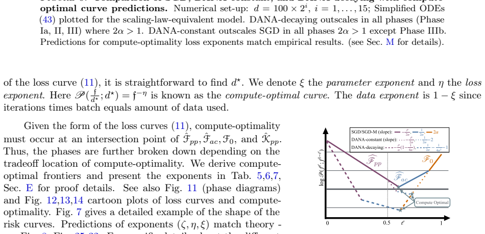
On the PLRF model, a random-features least-squares problem whose data-coordinate and target-coordinate decays are parameterized by $\alpha$ and $\beta$, the expected loss of any algorithm in the general momentum class (Gen-Mom-SGD) is shown to follow a Volterra equation whose forcing and kernel terms are controlled by two explicit measures, $\mu_F$ and $\mu_K$, arising from a deterministic equivalent of the random feature covariance. The main theorem states that under $2\alpha+2\beta>1$, $\alpha>1/4$, $\beta\le\alpha+1$, fixed batch size, and stability conditions, the loss obeys $P(t)\asymp \hat F(\vartheta(t))+\gamma \hat K_{pp}(\vartheta(t))$ with the time change $\vartheta(t)=1+2(\gamma_2+\gamma_3/\delta)Bt$ for SGD-M and $\vartheta(t)=1+2\gamma_2Bt+(\int_0^t\sqrt{\gamma_3(s)B}\,ds)^2$ for DANA. Consequently SGD-M has identical scaling-law exponents to SGD, since its effective learning rate is $\gamma_2+\gamma_3/\delta$, while the DANA time change accelerates the argument of the forcing function. With $\gamma_3(t)\asymp(1+t)^{-1/(2\alpha)}$, DANA-decaying outscales SGD for all regimes $t=d^{\ell}$, $0<\ell<2\alpha$, in the $2\alpha>1$ region, and the authors derive explicit compute-optimal parameter, loss, and data exponents showing that DANA's compute-optimal curve is not $d\asymp f^{1/2}$.
Load-bearing premise
The scaling-law exponents are proved for a simplified differential-equation model with a deterministic stand-in for the random covariance, not for the exact discrete stochastic momentum algorithm; if that reduction is unfaithful in some training regime, the predicted exponents may not describe the actual algorithm.
Editorial extensions
If this is right
- DANA-decaying with $\kappa_3=1/(2\alpha)$ gives strictly better loss exponents than SGD in every training regime $t=d^{\ell}$, $0<\ell<2\alpha$, for $2\alpha>1$, and is more sample-efficient and compute-efficient than both SGD and DANA-constant.
- SGD-M with any fixed momentum $\delta$ reproduces the SGD exponents exactly; its only effect is to replace $\gamma_2$ by the larger effective learning rate $\gamma_2+\gamma_3/\delta$.
- DANA-constant, with $\kappa_3=0$ and $\gamma_3\asymp\gamma_2/d$, behaves like SGD for $t\le d$ and outscales SGD for $1<\ell<2\alpha$, a regime that exists only when $2\alpha>1$.
- At compute-optimality for $2\alpha>1$, DANA-decaying never uses $d_\star(f)\asymp f^{1/2}$; depending on the phase it undertrains or overtrains relative to the Chinchilla ratio, and it lowers the compute-optimal loss exponent.
- On LSTMs trained on text, DANA-decaying's empirical loss exponents vary smoothly with $\kappa_3$, recover the predicted divergent, outscaling, and SGD-like regimes, and improve on SGD near $\kappa_3\approx0.7$.
Reading between the lines
- The effective-dimension interpretation suggests a test outside quadratics: estimate $\alpha$ from the spectral decay of a real dataset's covariance, set $\kappa_3=1/(2\alpha)$, and check whether the loss-exponent improvement persists; the paper treats this only as an open question.
- If DANA's gain carries over to preconditioned or adaptive optimizers, then Adam plus a DANA-style decaying momentum term could change exponents on real networks; the paper lists this as future work, so it is an extension, not a claim.
- The result implies empirical compute-optimal frontier fits should report the optimizer: two algorithms that differ only in momentum can have different $d_\star(f)$ exponents, so a single Chinchilla exponent is not an algorithm-independent constant.
- For $2\alpha<1$, all analyzed momentum variants collapse to SGD scaling, so the practical window for outscaling is precisely the regime where data power-law decay is strong enough; whether another algorithm can cross the high-dimensional line remains open.
Editorial analysis
A structured set of objections, weighed in public.
Referee Report
Summary. This paper studies scaling laws for stochastic momentum methods on the power law random features (PLRF) model. The authors derive a Poissonized ODE system (22) and an associated Volterra equation for the expected loss, then introduce a simplified ODE system (43) and replace the random spectral measures by deterministic equivalents (33). The main result, Theorem 3.1, states scaling laws of the form P(t) ≍ F(ϑ(t)) + γ Kpp(ϑ(t)) for SGD, classic momentum (SGD-M), and two DANA variants, with explicit time changes ϑ(t) and stability conditions. It is claimed that SGD-M matches SGD exponents while DANA-constant and DANA-decaying improve the loss exponents for 2α > 1, including in compute-optimal scaling. The theoretical predictions are tested on PLRF simulations and on LSTM language modeling (Fig. 2).
Significance. If the theorem applied to the exact discrete algorithms, this would be a significant contribution: it would show that dimension- and data-dependent momentum schedules can change the exponent of scaling laws, not merely the constant, and would provide principled compute-optimal training regimes that differ from the Chinchilla d⋆ ≍ f^{1/2} law. The derivation has a notable strength: the time change ϑ(t) in (9) contains no fitted constants, and the loss exponents are derived from the model rather than fitted to simulation, so the theory makes falsifiable predictions. The paper is also transparent about its two main reductions, the simplified ODE and the deterministic equivalent, and supports them with extensive numerical studies, including a large-scale LSTM experiment. The main weakness is that the proven scaling laws apply to the simplified ODE with the deterministic equivalent, not to the exact discrete algorithm as stated in the introduction, and some theorem hypotheses appear inconsistent with the broad claims made in the main text.
major comments (4)
- [Theorem 3.1, Remark C.3, §3.1] The scaling-law statements in Theorem 3.1 are proven for the solution of the simplified Volterra equation (58), which combines the simplified ODEs (43) with the deterministic equivalent measures (33)/(36), rather than for the exact discrete Gen-Mom-SGD algorithm introduced in (13). The exact ODE (22) contains additional terms of order Δ², γ3², γ1γ3, and λ², and Lemma C.1 justifies the simplified ODE only as a non-degenerate high-dimensional limit in which learning rates are scaled inversely with dimension; Remark C.3 explicitly states that the link between dropping those terms and the finite learning-rate regime used here (e.g., γ2 on the order of 1 for 2α > 1) is left for future work. The deterministic equivalent is also supported only numerically (Fig. 3c). Because the central outscaling claim is about the algorithm class Gen-Mom-SGD, the theorem as stated does not directly prove the headline claim; the PLRF experiments (e.g., Fig. 8) validate the simplified ODE against direct simulation, but do not compare the exact ODE (22) with the simplified ODE (43), so this key reduction is not tested. I recommend that the authors either prove the reduction, add a direct numerical comparison of (22) and (43) across the regimes used in the scaling laws, or explicitly restate the theorem's conclusions as being about the simplified model rather than the discrete algorithm.
- [Theorem 3.1, §4, Remark B.4] The recommended and headline choice for DANA-decaying is κ3 = 1/(2α) (Remark B.4, Section 4, Fig. 3), but the summarized Theorem 3.1 imposes the additional requirement (1/2α) < κ3 < 1 for DANA-decaying, which excludes κ3 = 1/(2α). The stability conditions listed just above the theorem do include a branch for κ3 ≥ 1/(2α), so the exclusion appears to be a mismatch rather than a deliberate boundary issue. If Theorem I.2 in the appendix covers the endpoint κ3 = 1/(2α), the main text needs to state that; otherwise the paper's optimal-schedule outscaling claim is not supported by the proved result. This is load-bearing because all of the DANA-decaying claims in the title and abstract rest on the endpoint schedule.
- [Theorem 3.1, §4, Fig. 6] Theorem 3.1 assumes β ≤ α + 1, yet the paper claims DANA-decaying outscales SGD for all (α, β) with 2α > 1 and presents compute-optimal experiments in Phase IIIa with α = 1.4, β = 3.0 (Fig. 6), which violates β ≤ α + 1 = 2.4. The authors note in Section C.4 that they believe α > 1/4 and α + 1 > β are proof artifacts, but as stated the theorem does not cover the regime shown in their own figure. Either the theorem should be extended to β > α + 1, or the claim of universal outscaling for 2α > 1 should be flagged as conjecture with a supporting argument.
- [Appendix B.2] The stability conditions in Theorem 3.1 are derived from the simplified ODEs, but the authors themselves warn that these can miss stability conditions of the original algorithm. In Appendix B.2, for SGD-M they observe that the simplified Volterra equation neglects Δ² terms, which makes any Δ > 0 appear convergent, and that the coin-flip ODEs (49) give an explicit condition 2δ(2−δ)/(2(2B+1)+δ(3B+1)) > γ3 > 0 with δ ∈ (0, 2). Since stability is a hypothesis of the scaling-law theorem, this discrepancy means the theorem may describe a regime that the actual algorithm does not enter. The LSTM sweep in Fig. 2a shows a divergence boundary near κ3 = 0.6, indicating the practical importance of getting the stability boundary right. The authors should reconcile the simplified-ODE stability conditions with the exact or coin-flip conditions, or at least verify by simulation that the stable set of the discrete algorithm contains the stable set claimed in the theorem.
minor comments (4)
- [Footnote 1] The definition of ≍ says the constants c and C are independent of d, but the scaling-law statements require comparison of functions of both t and d with constants uniform over the stated t-regimes; the definition should specify the full uniformity, e.g., independent of d and uniform in t over each scaling regime.
- [(5), (39), Theorem 3.1] The notation P(t) is used ambiguously: in (5) it is the expected loss of the discrete iterates, while in (39) and (58) it is the solution of the deterministic Volterra equation; Theorem 3.1 should state explicitly which object the ≍ bound refers to (Remark C.4 partially clarifies this, but not at the theorem statement).
- [Abstract, §3.1, Fig. 11] The abstract and Section 3 mention 'four distinct loss curve shapes', but the paper's phase diagrams (Fig. 11) contain subphases Ia, Ib, Ic, IIa, IIb, IIIa, IIIb, IVa, and IVb; the terminology should be aligned so that the reader can map the four shapes to the full phase structure.
- [Fig. 5] The colorbar label 'logd(time to reach irreducible loss)' is not informative about the base of the logarithm and whether it is per-algorithm or per-problem; please clarify the quantity being plotted.
Circularity Check
No circularity: the DANA exponents are derived from the PLRF Volterra/ODE model rather than fitted to the predicted loss exponents; the acknowledged model reductions are correctness risks, not circular steps.
full rationale
The paper's central derivation chain is self-contained in the sense required for a circularity audit: the scaling-law exponents and the outscaling claim are logical consequences of Theorem 3.1, which is proved from the simplified ODE system (43), the deterministic-equivalent measures (36)/(33), and the Volterra reduction (58). The DANA schedule is not fitted to the loss exponents it is said to predict. The hyperparameter κ3 = 1/(2α) is motivated by a spectral 'effective dimension' heuristic (Section 3, 'effective dimension at iteration t ≍ (tB)^{-1/(2α)}') and then independently proved, via Theorem 3.1 and the appendix, to produce better exponents; the paper's own sweeps in Fig. 3 are empirical confirmation, not the source of the theorem. Likewise, the constants γ2 = 1/(2 tr) and γ3 = (1/5)γ2 are chosen for stability and enter only as constants, not as fitted parameters in the exponent calculation. The comparison against LSTM loss exponents (Fig. 2) is a genuine external prediction: the theory fixes the relationship between κ3 and the expected improvement from the PLRF model, and the measured exponents are fit from runs, not fed back into the derivation. The only load-bearing imported result is the deterministic-equivalent analysis of the power-law random features covariance, attributed to [79] (whose authors overlap with the current paper). This is not circular: [79] is a separate published result with its own derivation, and the current paper's Appendix D strengthens and uses it to bound the measures µF and µK; the target result (DANA outscaling for the stable simplified dynamics) is not equivalent to that input by construction. The paper transparently flags two limitations: Remark C.3 states that the link between dropping higher-order ODE terms and the non-degenerate high-dimensional limit is left for future work, and the passage near Eq. (33) states that the PLRF deterministic-equivalent proof falls outside textbook RMT and is supported numerically (Fig. 3c). These are unproved modeling reductions that create correctness risk for the claim as a statement about the exact discrete algorithm, but they are not cases where a prediction reduces to a fitted input or to a self-citation by definition. No step in the derivation equates the predicted quantity with an input by construction, and therefore the appropriate circularity score is 0.
Assumptions & free parameters
free parameters (4)
- k3 (DANA-decaying time exponent) =
1/(2α) for optimality; theorem holds for κ3 in (1/(2α),1)
- k2 (DANA-constant dimension exponent) =
1 + κ1, with κ1 = max{0, 1-2α}
- Ratio γ̃3/γ2 =
1/5 (recommended), c2 = 0.5/Tr(D) in experiments
- Momentum decay constant δ =
δ = 8 for LSTM; δ > 4 max{(2α+2β-1)/α, 4-1/α} for PLRF
assumptions (5)
- domain assumption Power-law data and target (Assumption 1): data coordinates scale as j^{-α} and target coefficients as j^{-β}.
- domain assumption Zero initialization (Assumption 2): θ0 = 0 and y_{-1} = 0.
- ad hoc to paper Simplified ODEs (43) accurately model the risk curves of the discrete Gen-Mom-SGD algorithms.
- ad hoc to paper Deterministic equivalent (33) with measures μF, μK correctly represents the random matrix spectral measures.
- domain assumption Theorem conditions: 2α+2β>1, α>1/4, β≤α+1, and parameters not on critical lines.
Cite this review
Pith. "Pith review of Dimension-adapted Momentum Outscales SGD." pith.science (2026). https://pith.science/paper/BXOA6LOW
@misc{pith2026250516098,
  author       = {Pith},
  title        = {Pith review of: Dimension-adapted Momentum Outscales SGD},
  year         = {2026},
  howpublished = {\url{https://pith.science/paper/BXOA6LOW}},
  note         = {Machine review of arXiv:2505.16098}
}
read the original abstract
We investigate scaling laws for stochastic momentum algorithms with small batch on the power law random features model, parameterized by data complexity, target complexity, and model size. When trained with a stochastic momentum algorithm, our analysis reveals four distinct loss curve shapes determined by varying data-target complexities. While traditional stochastic gradient descent with momentum (SGD-M) yields identical scaling law exponents to SGD, dimension-adapted Nesterov acceleration (DANA) improves these exponents by scaling momentum hyperparameters based on model size and data complexity. This outscaling phenomenon, which also improves compute-optimal scaling behavior, is achieved by DANA across a broad range of data and target complexities, while traditional methods fall short. Extensive experiments on high-dimensional synthetic quadratics validate our theoretical predictions and large-scale text experiments with LSTMs show DANA's improved loss exponents over SGD hold in a practical setting.
Figures


Figures from the paper (38 more)




Forward citations
Cited by 1 Pith paper
-
On the Effectiveness of the z-Transform Method in Quadratic Optimization
Using z-transforms and Tauberian theory, this paper derives sharp asymptotic rates, such as 1/k^omega for gradient descent and 1/k^{min(2omega, omega+1)} for Nesterov acceleration, for quadratic optimization in infini...
Reference graph
Works this paper leans on
-
[1]
Martín Abadi, Ashish Agarwal, Paul Barham, Eugene Brevdo, Zhifeng Chen, Craig Citro, Greg S. Corrado, Andy Davis, Jeffrey Dean, Matthieu Devin, Sanjay Ghemawat, Ian Goodfellow, Andrew Harp, Geoffrey Irving, Michael Isard, Yangqing Jia, Rafal Jozefowicz, Lukasz Kaiser, Manjunath Kudlur, Josh Levenberg, Dandelion Mané, Rajat Monga, Sherry Moore, Derek Murra...
-
[2]
Katyusha: The first direct acceleration of stochastic gradient methods.The Journal of Machine Learning Research, 18(1):8194–8244, 2017
Zeyuan Allen-Zhu. Katyusha: The first direct acceleration of stochastic gradient methods.The Journal of Machine Learning Research, 18(1):8194–8244, 2017
2017
-
[3]
Zeyuan Allen-Zhu and Lorenzo Orecchia. Linear coupling: An ultimate unification of gradient and mirror descent.arXiv preprint arXiv:1407.1537, 2014
arXiv 2014
-
[4]
From high-dimensional & mean-field dynamics to dimensionless odes: A unifying approach to sgd in two-layers networks
Luca Arnaboldi, Ludovic Stephan, Florent Krzakala, and Bruno Loureiro. From high-dimensional & mean-field dynamics to dimensionless odes: A unifying approach to sgd in two-layers networks. InThe Thirty Sixth Annual Conference on Learning Theory (COLT), pages 1199–1227. PMLR, 2023
2023
-
[5]
Springer, 2003
Søren Asmussen, Soren Asmussen, and Sren Asmussen.Applied probability and queues, volume 2. Springer, 2003
2003
-
[6]
On the Convergence of Nesterov’s Accelerated Gradient Method in Stochastic Settings
Mahmoud Assran and Michael Rabbat. On the Convergence of Nesterov’s Accelerated Gradient Method in Stochastic Settings. InProceedings of the 37th International Conference on Machine Learning (ICML), 2020
2020
-
[7]
Alexander Atanasov, Blake Bordelon, Jacob A Zavatone-Veth, Courtney Paquette, and Cengiz Pehlevan. Two-Point Deterministic Equivalence for Stochastic Gradient Dynamics in Linear Models.arXiv preprint arXiv:2502.05074, 2025
arXiv 2025
-
[8]
Courier Corporation, 2004
Krishna B Athreya, Peter E Ney, and PE Ney.Branching processes. Courier Corporation, 2004
2004
Show all 138 references
-
[9]
Robust Accelerated Gradient Methods for Smooth Strongly Convex Functions.SIAM Journal on Optimization, 30(1):717– 751, 2020
Necdet Serhat Aybat, Alireza Fallah, Mert Gürbüzbalaban, and Asuman Ozdaglar. Robust Accelerated Gradient Methods for Smooth Strongly Convex Functions.SIAM Journal on Optimization, 30(1):717– 751, 2020
2020
-
[10]
High-dimensional analysis of double descent for linear regression with random projections
Francis Bach. High-dimensional analysis of double descent for linear regression with random projections. SIAM Journal on Mathematics of Data Science, 6(1):26–50, 2024
2024
-
[11]
Explaining neural scaling laws.Proc
Yasaman Bahri, Ethan Dyer, Jared Kaplan, Jaehoon Lee, and Utkarsh Sharma. Explaining neural scaling laws.Proc. Natl. Acad. Sci. USA, 121(27):Paper No. e2311878121, 8, 2024
2024
-
[12]
Springer, 2010
Zhidong Bai and Jack W Silverstein.Spectral analysis of large dimensional random matrices, volume 20. Springer, 2010
2010
-
[13]
Crowdsourcing with enhanced data quality assurance: An efficient approach to mitigate resource scarcity challenges in training large language models for healthcare
Prosanta Barai, Gondy Leroy, Prakash Bisht, Joshua M Rothman, Sumi Lee, Jennifer Andrews, Sydney A Rice, and Arif Ahmed. Crowdsourcing with enhanced data quality assurance: An efficient approach to mitigate resource scarcity challenges in training large language models for hea...
2024
-
[14]
Bartlett, Philip M
Peter L. Bartlett, Philip M. Long, Gábor Lugosi, and Alexander Tsigler. Benign overfitting in linear regression.Proc. Natl. Acad. Sci. USA, 117(48):30063–30070, 2020. 12 DIMENSION-ADAPTED MOMENTUM OUTSCALES SGD
2020
-
[15]
On the fast convergence of minibatch heavy ball momentum.IMA Journal of Numerical Analysis, page drae033, 08 2024
Raghu Bollapragada, Tyler Chen, and Rachel Ward. On the fast convergence of minibatch heavy ball momentum.IMA Journal of Numerical Analysis, page drae033, 08 2024
2024
-
[16]
A Dynamical Model of Neural Scaling Laws
Blake Bordelon, Alexander Atanasov, and Cengiz Pehlevan. A Dynamical Model of Neural Scaling Laws. InProceedings of the 41st International Conference on Machine Learning (ICML), volume 235 ofProceedings of Machine Learning Research, pages 4345–4382. PMLR, 2024
2024
-
[17]
How Feature Learning Can Improve Neural Scaling Laws .International Conference on Learning Representations (ICLR), 2025
Blake Bordelon, Alexander Atanasov, and Cengiz Pehlevan. How Feature Learning Can Improve Neural Scaling Laws .International Conference on Learning Representations (ICLR), 2025
2025
-
[18]
On ill-posed problems and the method of conjugate gradients
Helmut Brakhage. On ill-posed problems and the method of conjugate gradients. InInverse and Ill-Posed Problems, pages 165–175. Academic Press, 1987
1987
-
[19]
Language models are few-shot learners.Advances in neural information processing systems, 33:1877–1901, 2020
Tom Brown, Benjamin Mann, Nick Ryder, Melanie Subbiah, Jared D Kaplan, Prafulla Dhariwal, Arvind Neelakantan, Pranav Shyam, Girish Sastry, Amanda Askell, et al. Language models are few-shot learners.Advances in neural information processing systems, 33:1877–1901, 2020
1901
-
[20]
Accelerated Linear Convergence of Stochastic Momentum Methods in Wasserstein Distances
Bugra Can, Mert Gurbuzbalaban, and Lingjiong Zhu. Accelerated Linear Convergence of Stochastic Momentum Methods in Wasserstein Distances. InProceedings of the 36th International Conference on Machine Learning (ICML), volume 97, pages 891–901. Proceedings of Machine Learning Re...
2019
-
[21]
Optimal rates for the regularized least-squares algorithm
Andrea Caponnetto and Ernesto De Vito. Optimal rates for the regularized least-squares algorithm. Foundations of Computational Mathematics, 7:331–368, 2007
2007
-
[22]
Learning with sgd and random features
Luigi Carratino, Alessandro Rudi, and Lorenzo Rosasco. Learning with sgd and random features. Advances in Neural Information Processing Systems (NeurIPS), 31, 2018
2018
-
[23]
Dimension free ridge regression.arXiv preprint arXiv:2210.08571, 2022
Chen Cheng and Andrea Montanari. Dimension free ridge regression.arXiv preprint arXiv:2210.08571, 2022
2022 arXiv
-
[24]
Coddington and Norman Levinson.Theory of ordinary differential equations
Earl A. Coddington and Norman Levinson.Theory of ordinary differential equations. McGraw-Hill Book Company, Inc., New York-Toronto-London, 1955
1955
-
[25]
Hitting the high-dimensional notes: an ODE for SGD learning dynamics on GLMs and multi-index models.Inf
Elizabeth Collins-Woodfin, Courtney Paquette, Elliot Paquette, and Inbar Seroussi. Hitting the high-dimensional notes: an ODE for SGD learning dynamics on GLMs and multi-index models.Inf. Inference, 13(4):Paper No. iaae028, 107, 2024
2024
-
[26]
The High Line: Exact Risk and Learning Rate Curves of Stochastic Adaptive Learning Rate Algorithms
Elizabeth Collins-Woodfin, Inbar Seroussi, Begoña García Malaxechebarría, Andrew W Mackenzie, Elliot Paquette, and Courtney Paquette. The High Line: Exact Risk and Learning Rate Curves of Stochastic Adaptive Learning Rate Algorithms. InAdvances in Neural Information Processing...
2024
-
[27]
Cambridge University Press, 2022
Romain Couillet and Zhenyu Liao.Random Matrix Methods for Machine Learning. Cambridge University Press, 2022
2022
-
[28]
Generalization Error Rates in Kernel Regression: The Crossover from the Noiseless to Noisy Regime.Advances in Neural Information Processing Systems (NeurIPS), 34, 2021
Hugo Cui, Bruno Loureiro, Florent Krzakala, and Lenka Zdeborová. Generalization Error Rates in Kernel Regression: The Crossover from the Noiseless to Noisy Regime.Advances in Neural Information Processing Systems (NeurIPS), 34, 2021
2021
-
[29]
(Accelerated) Noise-adaptive Stochastic Heavy-Ball Momentum.Transactions on Machine Learning Research (TMLR), 2025
Anh Quang Dang, Reza Babanezhad Harikandeh, and Sharan Vaswani. (Accelerated) Noise-adaptive Stochastic Heavy-Ball Momentum.Transactions on Machine Learning Research (TMLR), 2025
2025
-
[30]
On the interplay between data structure and loss function in classification problems.Advances in Neural Information Processing Systems (NeurIPS), 34:8506–8517, 2021
Stéphane d’Ascoli, Marylou Gabrié, Levent Sagun, and Giulio Biroli. On the interplay between data structure and loss function in classification problems.Advances in Neural Information Processing Systems (NeurIPS), 34:8506–8517, 2021
2021
-
[31]
The DeepMind JAX Ecosystem.http://github.com/google-deepmind, 2020
DeepMind, IgorBabuschkin, KateBaumli, AlisonBell, SuryaBhupatiraju, JakeBruce, PeterBuchlovsky, David Budden, Trevor Cai, Aidan Clark, Ivo Danihelka, Antoine Dedieu, Claudio Fantacci, Jonathan Godwin, Chris Jones, Ross Hemsley, Tom Hennigan, Matteo Hessel, Shaobo Hou, Steven K...
2020
-
[32]
The Road Less Scheduled
Aaron Defazio, Xingyu Yang, Harsh Mehta, Konstantin Mishchenko, Ahmed Khaled, and Ashok Cutkosky. The Road Less Scheduled. InAdvances in Neural Information Processing Systems (NeurIPS), volume 37, pages 9974–10007, 2024
2024
-
[33]
Dimension-free deterministic equiva- lents and scaling laws for random feature regression
Leonardo Defilippis, Bruno Loureiro, and Theodor Misiakiewicz. Dimension-free deterministic equiva- lents and scaling laws for random feature regression. InAdvances in Neural Information Processing DIMENSION-ADAPTED MOMENTUM OUTSCALES SGD 13 Systems (NeurIPS), volume 37, pages...
2024
-
[34]
Optimal Distributed Online Prediction Using Mini-Batches.Journal of Machine Learning Research (JMLR), 13(1), 2012
Ofer Dekel, Ran Gilad-Bachrach, Ohad Shamir, and Lin Xiao. Optimal Distributed Online Prediction Using Mini-Batches.Journal of Machine Learning Research (JMLR), 13(1), 2012
2012
-
[35]
Nonparametric stochastic approximation with large step-sizes
Aymeric Dieuleveut and Francis Bach. Nonparametric stochastic approximation with large step-sizes. The Annals of Statistics, 44(4):1363 – 1399, 2016
2016
-
[36]
NIST Digital Library of Mathematical Functions.https://dlmf.nist.gov/, Release 1.2.4 of 2025-03-
2025
-
[37]
F. W. J. Olver, A. B. Olde Daalhuis, D. W. Lozier, B. I. Schneider, R. F. Boisvert, C. W. Clark, B. R. Miller, B. V. Saunders, H. S. Cohl, and M. A. McClain, eds
-
[38]
Continuized Accelerations of Deterministic and Stochastic Gradient Descents, and of Gossip Algorithms
Mathieu Even, Raphaël Berthier, Francis Bach, Nicolas Flammarion, Hadrien Hendrikx, Pierre Gaillard, Laurent Massoulié, and Adrien Taylor. Continuized Accelerations of Deterministic and Stochastic Gradient Descents, and of Gossip Algorithms. In M. Ranzato, A. Beygelzimer, Y. D...
2021
-
[39]
Scaling Exponents Across Parameterizations and Optimizers
Katie E Everett, Lechao Xiao, Mitchell Wortsman, Alexander A Alemi, Roman Novak, Peter J Liu, Izzeddin Gur, Jascha Sohl-Dickstein, Leslie Pack Kaelbling, Jaehoon Lee, et al. Scaling Exponents Across Parameterizations and Optimizers. InInternational Conference on Machine Learni...
2024
-
[40]
From Averaging to Acceleration, There is Only a Step-size
Nicolas Flammarion and Francis Bach. From Averaging to Acceleration, There is Only a Step-size. In Proceedings of The 28th Conference on Learning Theory (COLT), volume 40 ofProceedings of Machine Learning Research, pages 658–695. PMLR, 03–06 Jul 2015
2015
-
[41]
Stochastic Heavy Ball.arXiv preprints arXiv:1609.04228, 2016
Sèbastien Gadat, Fabien Panloup, and Sofiane Saadane. Stochastic Heavy Ball.arXiv preprints arXiv:1609.04228, 2016
2016 arXiv
-
[42]
Rigorous dynamical mean-field theory for stochastic gradient descent methods.SIAM Journal on Mathematics of Data Science, 6(2):400–427, 2024
Cedric Gerbelot, Emanuele Troiani, Francesca Mignacco, Florent Krzakala, and Lenka Zdeborova. Rigorous dynamical mean-field theory for stochastic gradient descent methods.SIAM Journal on Mathematics of Data Science, 6(2):400–427, 2024
2024
-
[43]
Optimal stochastic approximation algorithms for strongly convex stochastic composite optimization I: A generic algorithmic framework.SIAM J
Saeed Ghadimi and Guanghui Lan. Optimal stochastic approximation algorithms for strongly convex stochastic composite optimization I: A generic algorithmic framework.SIAM J. Optim., 22(4):1469–1492, 2012
2012
-
[44]
Optimal stochastic approximation algorithms for strongly convex stochastic composite optimization, II: Shrinking procedures and optimal algorithms.SIAM J
Saeed Ghadimi and Guanghui Lan. Optimal stochastic approximation algorithms for strongly convex stochastic composite optimization, II: Shrinking procedures and optimal algorithms.SIAM J. Optim., 23(4):2061–2089, 2013
2013
-
[45]
On the resolvents of nonconvolution Volterra kernels.Funkcial
Gustaf Gripenberg. On the resolvents of nonconvolution Volterra kernels.Funkcial. Ekvac., 23(1):83–95, 1980
1980
-
[46]
Siegel, and Stephan Wojtowytsch
Kanan Gupta, Jonathan W. Siegel, and Stephan Wojtowytsch. Nesterov acceleration despite very noisy gradients. InAdvances in Neural Information Processing Systems (NeurIPS), volume 37, pages 20694–20744, 2024
2024
-
[47]
Deterministic equivalents for certain functionals of large random matrices.Ann
Walid Hachem, Philippe Loubaton, and Jamal Najim. Deterministic equivalents for certain functionals of large random matrices.Ann. Appl. Probab., 17(3):875–930, 2007
2007
-
[48]
Deep learning scaling is predictable, empirically
Joel Hestness, Sharan Narang, Newsha Ardalani, Gregory Diamos, Heewoo Jun, Hassan Kianinejad, Md Mostofa Ali Patwary, Yang Yang, and Yanqi Zhou. Deep learning scaling is predictable, empirically. arXiv preprint arXiv:1712.00409, 2017
2017 arXiv
-
[49]
Long short-term memory.Neural computation, 9(8):1735– 1780, 1997
Sepp Hochreiter and Jürgen Schmidhuber. Long short-term memory.Neural computation, 9(8):1735– 1780, 1997
1997
-
[50]
An empirical analysis of compute-optimal large language model training
Jordan Hoffmann, Sebastian Borgeaud, Arthur Mensch, Elena Buchatskaya, Trevor Cai, Eliza Ruther- ford, Diego de Las Casas, Lisa Anne Hendricks, Johannes Welbl, Aidan Clark, Tom Hennigan, Eric Noland, Katie Millican, George van den Driessche, Bogdan Damoc, Aurelia Guy, Simon Os...
2022
-
[51]
Lu, and Theodor Misiakiewicz
Hong Hu, Yue M. Lu, and Theodor Misiakiewicz. Asymptotics of Random Feature Regression Beyond the Linear Scaling Regime.arXiv preprint arXiv:2403.08160, 2024
2024 arXiv
-
[52]
Accelerating Stochastic Gradient Descent for Least Squares Regression
Prateek Jain, Sham Kakade, Rahul Kidambi, Praneeth Netrapalli, and Aaron Sidford. Accelerating Stochastic Gradient Descent for Least Squares Regression. InProceedings of the 31st Conference On Learning Theory (COLT), volume 75, pages 545–604, 2018. 14 DIMENSION-ADAPTED MOMENTU...
2018
-
[53]
Exploring the limits of language modeling.arXiv preprint arXiv:1602.02410, 2016
Rafal Jozefowicz, Oriol Vinyals, Mike Schuster, Noam Shazeer, and Yonghui Wu. Exploring the limits of language modeling.arXiv preprint arXiv:1602.02410, 2016
2016 arXiv
-
[54]
Brown, Benjamin Chess, Rewon Child, Scott Gray, Alex Radford, Jeffrey Wu, and Dario Amodei
Jared Kaplan, Sam McCandlish, Tom Henighan, Tom B. Brown, Benjamin Chess, Rewon Child, Scott Gray, Alex Radford, Jeffrey Wu, and Dario Amodei. Scaling laws for neural language models.arXiv preprint arXiv:2001.08361, 2020
2001 arXiv
-
[55]
On the Insufficiency of Existing Momentum Schemes for Stochastic Optimization
Rahul Kidambi, Praneeth Netrapalli, Prateek Jain, and Sham Kakade. On the Insufficiency of Existing Momentum Schemes for Stochastic Optimization. In2018 Information Theory and Applications Workshop (ITA), pages 1–9, 2018
2018
-
[56]
Adam: A method for stochastic optimization.International Conference on Learning Representations (ICLR), 2015
Diederik P Kingma and Jimmy Ba. Adam: A method for stochastic optimization.International Conference on Learning Representations (ICLR), 2015
2015
-
[57]
Sentencepiece: A simple and language independent subword tokenizer and detokenizer for neural text processing.arXiv preprint arXiv:1808.06226, 2018
Taku Kudo and John Richardson. Sentencepiece: A simple and language independent subword tokenizer and detokenizer for neural text processing.arXiv preprint arXiv:1808.06226, 2018
2018 arXiv
-
[58]
A Generic Acceleration Framework for Stochastic Composite Optimization
Andrei Kulunchakov and Julien Mairal. A Generic Acceleration Framework for Stochastic Composite Optimization. InAdvances in Neural Information Processing Systems (NeurIPS), volume 32, 2019
2019
-
[59]
A Lyapunov analysis for accelerated gradient methods: from deterministic to stochastic case
Maxime Laborde and Adam Oberman. A Lyapunov analysis for accelerated gradient methods: from deterministic to stochastic case. InProceedings of the Twenty Third International Conference on Artificial Intelligence and Statistics (AISTATS), volume 108, pages 602–612. Proceedings ...
2020
-
[60]
Trajectory of mini-batch momentum: batch size saturation and convergence in high dimensions.Advances in Neural Information Processing Systems (NeurIPS), 35:36944–36957, 2022
Kiwon Lee, Andrew Cheng, Elliot Paquette, and Courtney Paquette. Trajectory of mini-batch momentum: batch size saturation and convergence in high dimensions.Advances in Neural Information Processing Systems (NeurIPS), 35:36944–36957, 2022
2022
-
[61]
Risk bounds of accelerated SGD for overparameterized linear regression.arXiv preprint arXiv:2311.14222, 2023
Xuheng Li, Yihe Deng, Jingfeng Wu, Dongruo Zhou, and Quanquan Gu. Risk bounds of accelerated SGD for overparameterized linear regression.arXiv preprint arXiv:2311.14222, 2023
2023 arXiv
-
[62]
Zhenyu Liao, Romain Couillet, and Mahoney Mahoney. A Random Matrix Analysis of Random Fourier Features: Beyond the Gaussian Kernel, a Precise Phase Transition, and the Corresponding Double Descent.arXiv preprint arXiv:2006.05013, 2020
2006 arXiv
-
[63]
Kakade, Peter L
Licong Lin, Jingfeng Wu, Sham M. Kakade, Peter L. Bartlett, and Jason D. Lee. Scaling Laws in Linear Regression: Compute, Parameters, and Data. InAdvances in Neural Information Processing Systems (NeurIPS), volume 37, pages 60556–60606. Curran Associates, Inc., 2024
2024
-
[64]
Accelerating SGD with momentum for over-parameterized learning
Chaoyue Liu and Mikhail Belkin. Accelerating SGD with momentum for over-parameterized learning. InProceedings of the 37th International Conference on Machine Learning (ICML), 2020
2020
-
[65]
Liu, Roman Novak, Jaehoon Lee, Mitchell Wortsman, Lechao Xiao, Katie Everett, Alexander A
Peter J. Liu, Roman Novak, Jaehoon Lee, Mitchell Wortsman, Lechao Xiao, Katie Everett, Alexander A. Alemi, Mark Kurzeja, Pierre Marcenac, Izzeddin Gur, Simon Kornblith, Kelvin Xu, Gamaleldin Elsayed, Ian Fischer, Jeffrey Pennington, Ben Adlam, and Jascha-Sohl Dickstein. Nanodo...
2024
-
[66]
Optimal Algorithms in Linear Regression under Covariate Shift: On the Importance of Precondition.arXiv preprint arXiv:2502.09047, 2025
Yuanshi Liu, Haihan Zhang, Qian Chen, and Cong Fang. Optimal Algorithms in Linear Regression under Covariate Shift: On the Importance of Precondition.arXiv preprint arXiv:2502.09047, 2025
2025 arXiv
-
[67]
Momentum and stochastic momentum for stochastic gradient, Newton, proximal point and subspace descent methods.Comput
Nicolas Loizou and Peter Richtárik. Momentum and stochastic momentum for stochastic gradient, Newton, proximal point and subspace descent methods.Comput. Optim. Appl., 77(3):653–710, 2020
2020
-
[68]
Learning curves of generic features maps for realistic datasets with a teacher-student model.Advances in Neural Information Processing Systems (NeurIPS), 34:18137–18151, 2021
Bruno Loureiro, Cedric Gerbelot, Hugo Cui, Sebastian Goldt, Florent Krzakala, Marc Mezard, and Lenka Zdeborová. Learning curves of generic features maps for realistic datasets with a teacher-student model.Advances in Neural Information Processing Systems (NeurIPS), 34:18137–18...
2021
-
[69]
Roberts, and James Sully
Alexander Maloney, Daniel A. Roberts, and James Sully. A Solvable Model of Neural Scaling Laws. arXiv preprint arXiv:2210.16859, 2024
2024 arXiv
-
[70]
An empirical model of large-batch training.arXiv preprint arXiv:1812.06162, 2018
Sam McCandlish, Jared Kaplan, Dario Amodei, and OpenAI Dota Team. An empirical model of large-batch training.arXiv preprint arXiv:1812.06162, 2018
2018 arXiv
-
[71]
The generalization error of random features regression: Precise asymptotics and the double descent curve.Communications on Pure and Applied Mathematics, 75(4):667–766, 2022
Song Mei and Andrea Montanari. The generalization error of random features regression: Precise asymptotics and the double descent curve.Communications on Pure and Applied Mathematics, 75(4):667–766, 2022
2022
-
[72]
Anisotropic random feature regression in high dimensions
Gabriel Mel and Jeffrey Pennington. Anisotropic random feature regression in high dimensions. In International Conference on Learning Representations, 2021
2021
-
[73]
Connections between Schedule-Free Optimizers, AdEMAMix, and Accelerated SGD Variants.arXiv preprint arXiv:2502.02431, 2025
Depen Morwani, Nikhil Vyas, Hanlin Zhang, and Sham Kakade. Connections between Schedule-Free Optimizers, AdEMAMix, and Accelerated SGD Variants.arXiv preprint arXiv:2502.02431, 2025. DIMENSION-ADAPTED MOMENTUM OUTSCALES SGD 15
2025 arXiv
-
[74]
Yoonsoo Nam, Nayara Fonseca, Seok Hyeong Lee, Chris Mingard, and Ard A. Louis. An exactly solvable model for emergence and scaling laws in the multitask sparse parity problem. InAdvances in Neural Information Processing Systems (NeurIPS), volume 37, pages 39632–39693, 2024
2024
-
[75]
Springer, 2004
Yuri Nesterov.Introductory lectures on convex optimization. Springer, 2004
2004
-
[76]
The Role of Memory in Stochastic Optimization
Antonio Orvieto, Jonas Kohler, and Aurelien Lucchi. The Role of Memory in Stochastic Optimization. InProceedings of The 35th Uncertainty in Artificial Intelligence Conference, volume 115 ofProceedings of Machine Learning Research, pages 356–366, 2020
2020
-
[77]
SGD in the Large: Average-case Analysis, Asymptotics, and Stepsize Criticality
Courtney Paquette, Kiwon Lee, Fabian Pedregosa, and Elliot Paquette. SGD in the Large: Average-case Analysis, Asymptotics, and Stepsize Criticality. InProceedings of Thirty Fourth Conference on Learning Theory (COLT), volume 134, pages 3548–3626, 2021
2021
-
[78]
Dynamics of stochastic momentum methods on large-scale, quadratic models.Advances in Neural Information Processing Systems (NeurIPS), 34:9229–9240, 2021
Courtney Paquette and Elliot Paquette. Dynamics of stochastic momentum methods on large-scale, quadratic models.Advances in Neural Information Processing Systems (NeurIPS), 34:9229–9240, 2021
2021
-
[79]
Homogenization of SGD in high-dimensions: exact dynamics and generalization properties.arXiv preprint arXiv:2205.07069, 2022
Courtney Paquette, Elliot Paquette, Ben Adlam, and Jeffrey Pennington. Homogenization of SGD in high-dimensions: exact dynamics and generalization properties.arXiv preprint arXiv:2205.07069, 2022
2022 arXiv
-
[80]
4+3 Phases of Compute- Optimal Neural Scaling Laws
Elliot Paquette, Courtney Paquette, Lechao Xiao, and Jeffrey Pennington. 4+3 Phases of Compute- Optimal Neural Scaling Laws. InAdvances in Neural Information Processing Systems (NeurIPS), volume 37, 2024
2024
-
[81]
Statistical optimality of stochastic gradient descent on hard learning problems through multiple passes.Advances in Neural Information Processing Systems (NeurIPS), 31, 2018
Loucas Pillaud-Vivien, Alessandro Rudi, and Francis Bach. Statistical optimality of stochastic gradient descent on hard learning problems through multiple passes.Advances in Neural Information Processing Systems (NeurIPS), 31, 2018
2018
-
[82]
B.T. Polyak. Some methods of speeding up the convergence of iteration methods.USSR Computational Mathematics and Mathematical Physics, 04, 1964
1964
-
[83]
Resolving Discrepancies in Compute-Optimal Scaling of Language Models
Tomer Porian, Mitchell Wortsman, Jenia Jitsev, Ludwig Schmidt, and Yair Carmon. Resolving Discrepancies in Compute-Optimal Scaling of Language Models. InAdvances in Neural Information Processing Systems (NeurIPS), volume 37, pages 100535–100570, 2024
2024
-
[84]
Exploring the limits of transfer learning with a unified text-to-text transformer.Journal of machine learning research, 21(140):1–67, 2020
Colin Raffel, Noam Shazeer, Adam Roberts, Katherine Lee, Sharan Narang, Michael Matena, Yanqi Zhou, Wei Li, and Peter J Liu. Exploring the limits of transfer learning with a unified text-to-text transformer.Journal of machine learning research, 21(140):1–67, 2020
2020
-
[85]
Generalization properties of learning with random features
Alessandro Rudi and Lorenzo Rosasco. Generalization properties of learning with random features. Advances in Neural Information Processing Systems (NeurIPS), 30, 2017
2017
-
[86]
Almost sure convergence rates for Stochastic Gradient Descent and Stochastic Heavy Ball
Othmane Sebbouh, Robert M Gower, and Aaron Defazio. Almost sure convergence rates for Stochastic Gradient Descent and Stochastic Heavy Ball. InProceedings of Thirty Fourth Conference on Learning Theory, volume 134, pages 3935–3971. Proceedings of Machine Learning Research (PMLR), 2021
2021
-
[87]
Shallue, J
C.J. Shallue, J. Lee, J. Antognini, J. Sohl-Dickstein, R. Frostig, and G.E. Dahl. Measuring the Effects of Data Parallelism on Neural Network Training.Journal of Machine Learning Research, 20:1–49, 2019
2019
-
[88]
Stochastic gradient descent for non-smooth optimization: Convergence results and optimal averaging schemes
Ohad Shamir and Tong Zhang. Stochastic gradient descent for non-smooth optimization: Convergence results and optimal averaging schemes. InInternational conference on machine learning, pages 71–79. PMLR, 2013
2013
-
[89]
Scaling Laws from the Data Manifold Dimension.Journal of Machine Learning Research (JMLR), 23(9):1–34, 2022
Utkarsh Sharma and Jared Kaplan. Scaling Laws from the Data Manifold Dimension.Journal of Machine Learning Research (JMLR), 23(9):1–34, 2022
2022
-
[90]
On the empirical distribution of eigenvalues of a class of large dimensional random matrices.Journal of Multivariate analysis, 54(2):175–192, 1995
Jack W Silverstein and Zhi Dong Bai. On the empirical distribution of eigenvalues of a class of large dimensional random matrices.Journal of Multivariate analysis, 54(2):175–192, 1995
1995
-
[91]
Simon, Dhruva Karkada, Nikhil Ghosh, and Mikhail Belkin
James B. Simon, Dhruva Karkada, Nikhil Ghosh, and Mikhail Belkin. More is better in modern machine learning: when infinite overparameterization is optimal and overfitting is obligatory. InInternational Conference on Learning Representations (ICLR), 2024
2024
-
[92]
Weijie Su, Stephen Boyd, and Emmanuel J. Candès. A Differential Equation for Modeling Nesterov’s Accelerated Gradient Method: Theory and Insights.Journal of Machine Learning Research, 17(153):1– 43, 2016
2016
-
[93]
On the importance of initialization and momentum in deep learning
Ilya Sutskever, James Martens, George Dahl, and Geoffrey Hinton. On the importance of initialization and momentum in deep learning. InProceedings of the 30th International Conference on Machine Learning (ICML), volume 28, pages 1139–1147, 2013
2013
-
[94]
Accelerated sgd for non-strongly-convex least squares
Aditya Varre and Nicolas Flammarion. Accelerated sgd for non-strongly-convex least squares. In Proceedings of Thirty Fifth Conference on Learning Theory (COLT), volume 135 ofProceedings of Machine Learning Research, pages 2062–2126, 2022. 16 DIMENSION-ADAPTED MOMENTUM OUTSCALES SGD
2022
-
[95]
Last iterate convergence of SGD for Least-Squares in the Interpolation regime
Aditya Vardhan Varre, Loucas Pillaud-Vivien, and Nicolas Flammarion. Last iterate convergence of SGD for Least-Squares in the Interpolation regime. InAdvances in Neural Information Processing Systems (NeurIPS), volume 34, pages 21581–21591, 2021
2021
-
[96]
Fast and Faster Convergence of SGD for Over- Parameterized Models and an Accelerated Perceptron
Sharan Vaswani, Francis Bach, and Mark Schmidt. Fast and Faster Convergence of SGD for Over- Parameterized Models and an Accelerated Perceptron. InProceedings of the Twenty-Second International Conference on Artificial Intelligence and Statistics (ICML), volume 89 ofProceeding...
2019
-
[97]
Will we run out of data? Limits of LLM scaling based on human-generated data.arXiv preprint arXiv:2211.04325, 2022
Pablo Villalobos, Anson Ho, Jaime Sevilla, Tamay Besiroglu, Lennart Heim, and Marius Hobbhahn. Will we run out of data? Limits of LLM scaling based on human-generated data.arXiv preprint arXiv:2211.04325, 2022
2022 arXiv
-
[98]
Re-examining Double Descent and Scal- ing Laws under Norm-based Capacity via Deterministic Equivalence.arXiv preprint arXiv:2502.01585, 2025
Yichen Wang, Yudong Chen, Lorenzo Rosasco, and Fanghui Liu. Re-examining Double Descent and Scal- ing Laws under Norm-based Capacity via Deterministic Equivalence.arXiv preprint arXiv:2502.01585, 2025
2025
-
[99]
A variational perspective on accelerated methods in optimization.proceedings of the National Academy of Sciences, 113(47):E7351–E7358, 2016
Andre Wibisono, Ashia C Wilson, and Michael I Jordan. A variational perspective on accelerated methods in optimization.proceedings of the National Academy of Sciences, 113(47):E7351–E7358, 2016
2016
-
[100]
Small-scale proxies for large-scale Transformer training instabilities
Mitchell Wortsman, Peter J Liu, Lechao Xiao, Katie E Everett, Alexander A Alemi, Ben Adlam, John D Co-Reyes, Izzeddin Gur, Abhishek Kumar, Roman Novak, et al. Small-scale proxies for large-scale Transformer training instabilities. InThe Twelfth International Conference on Lear...
2023
-
[101]
Last Iterate Risk Bounds of SGD with Decaying Stepsize for Overparameterized Linear Regression
Jingfeng Wu, Difan Zou, Vladimir Braverman, Quanquan Gu, and Sham Kakade. Last Iterate Risk Bounds of SGD with Decaying Stepsize for Overparameterized Linear Regression. InProceedings of the 39th International Conference on Machine Learning (ICML), volume 162 ofProceedings of ...
2022
-
[102]
A Unified Analysis of Stochastic Momentum Methods for Deep Learning
Yan Yan, Tianbao Yang, Zhe Li Li, Qihang Lin, and Yi Yang. A Unified Analysis of Stochastic Momentum Methods for Deep Learning. InProceedings of the Twenty-Seventh International Joint Conference on Artificial Intelligence, IJCAI-18, pages 2955–2961. International Joint Confere...
2018
-
[103]
Tensor programs iv: Feature learning in infinite-width neural networks
Greg Yang and Edward J Hu. Tensor programs iv: Feature learning in infinite-width neural networks. InInternational Conference on Machine Learning, pages 11727–11737. PMLR, 2021
2021
-
[104]
Tensor programs V: tuning large neural networks via zero-shot hyperparameter transfer
Greg Yang, Edward J Hu, Igor Babuschkin, Szymon Sidor, Xiaodong Liu, David Farhi, Nick Ryder, Jakub Pachocki, Weizhu Chen, and Jianfeng Gao. Tensor programs V: tuning large neural networks via zero-shot hyperparameter transfer. InProceedings of the 35th International Conferenc...
2021
-
[105]
Tensor programs ivb: Adaptive optimization in the infinite-width limit
Greg Yang and Etai Littwin. Tensor programs ivb: Adaptive optimization in the infinite-width limit. arXiv preprint arXiv:2308.01814, 2023
2023 arXiv
-
[106]
Corner Gradient Descent.arXiv preprint arXiv:2504.12519, 2025
Dmitry Yarotsky. Corner Gradient Descent.arXiv preprint arXiv:2504.12519, 2025
2025 arXiv
-
[107]
SGD with Memory: Fundamental Properties and Stochastic Acceleration.International Conference on Learning Representations (ICLR), 2025
Dmitry Yarotsky and Maksim Velikanov. SGD with Memory: Fundamental Properties and Stochastic Acceleration.International Conference on Learning Representations (ICLR), 2025
2025
-
[108]
Which Algorithmic Choices Matter at Which Batch Sizes? Insights From a Noisy Quadratic Model
Guodong Zhang, Lala Li, Zachary Nado, James Martens, Sachdeva Sachdeva, George Dahl, Christopher Shallue, and Roger Grosse. Which Algorithmic Choices Matter at Which Batch Sizes? Insights From a Noisy Quadratic Model. InAdvances in Neural Information Processing Systems (NeurIP...
2019
-
[109]
Hanlin Zhang, Depen Morwani, Nikhil Vyas, Jingfeng Wu, Difan Zou, Udaya Ghai, Dean Foster, and Sham M. Kakade. How Does Critical Batch Size Scale in Pre-training? .International Conference on Learning Representations (ICLR), 2025
2025
-
[110]
Foster, and Sham Kakade
Difan Zou, Jingfeng Wu, Vladimir Braverman, Quanguan Gu, Dean P. Foster, and Sham Kakade. The Benefits of Implicit Regularization from SGD in Least Squares Problems (NeurIPS). InAdvances in Neural Information Processing Systems, volume 34, pages 5456–5468, 2021
2021
-
[111]
Benign overfitting of constant-stepsize SGD for linear regression.Journal of Machine Learning Research, 24(326):1–58, 2023
Difan Zou, Jingfeng Wu, Vladimir Braverman, Quanquan Gu, and Sham M Kakade. Benign overfitting of constant-stepsize SGD for linear regression.Journal of Machine Learning Research, 24(326):1–58, 2023. DIMENSION-ADAPTED MOMENTUM OUTSCALES SGD 17 Appendix: Dimension-adapted Momen...
2023
-
[112]
The power law random features model (PLRF) 4 18 DIMENSION-ADAPTED MOMENTUM OUTSCALES SGD
-
[113]
Scaling laws for SGD on the PLRF
Continuized analysis of general stochastic momentum algorithms 4 3.1. Scaling laws for SGD on the PLRF. 5
-
[114]
hidden-manifold
Using Momentum to outscale SGD 8 4.1. Compute-optimal regime. 8 References 11 Appendix A. Related Work 20 Appendix B. Additional Algorithm Set-up 23 B.1. Stochastic gradient descent (SGD) 23 B.2. Classic (constant) momentum (SGD-M) 26 B.3. Dimension-Adapted Nesterov Accelerati...
-
[115]
high-dimensional
By hitting both sides byΣVT, we get that ΣV T VΣ T U T D1/2 ˙b= 0⇒ΣΣ T U T D1/2 ˙b= 0. Thus for all nonzero singular valuesσj (or equivalently for all nonzero eigenvaluesλj of ˇK = W T DW), uT j D1/2 ˙b= 0. Additionally, we have that W T D1/2uj =VΣ T U T uj =VΣ T ej =σ jV ej =...
-
[116]
We denoteγ def =γ 2 + γ3 δ for classic momentum andγ def =γ 2 for both DANA algorithms and SGD
For various assumptions specific to the individual algorithms, there exists anM > 0large enough and constants ˜C(α, β, M,alg),˜c(α, β, M,alg)such that if γBt > Mthen: (62)˜c× F(t) + 1 γB K(t) ≤P(t)≤ ˜C× F(t) + 1 γB K(t) . We denoteγ def =γ 2 + γ3 δ for classic momentum andγ de...
-
[117]
Proposition D.2(Upper bound for large σ’s).Let α >0
□ This implies a first bound on the mass ofµF for largeσ. Proposition D.2(Upper bound for large σ’s).Let α >0. Suppose2 α + 2β >1. Then there is a constant C(α, β)such that∀M >0,we have µF([M,+∞])≤C(α, β). Additionally, for anyϵ >0, there exists somed >0such that∀d≥ d,µ F([1 +...
-
[118]
There exists M, ˜C depending only onαsuch that for anyC∈[d −2αM, 1 M ], we have: µK([C,2C])≤ ˜C×C 2− 1 2α . Proof. Using Lemma D.2, we only need to estimate1 π Im((x + iη)(1 −m (x + iη))d)for x∈ [d−2αM, 1 M ]and η(x) = (log(1/ϵ)/c) max{x1+1/(2α), π 2α x1−1/(2α) d }. Applying [...
-
[119]
On the other hand , ifα > 3 4, we haveFpp(t) = Fac(t)for t≍f 1/2+α 3/2+α but the optimal is to taket⋆ the largest
= f− (2α+2β−1) 3β+α . On the other hand , ifα > 3 4, we haveFpp(t) = Fac(t)for t≍f 1/2+α 3/2+α but the optimal is to taket⋆ the largest. This brings us to the second case. Fac(t) =F 0(t): We apply Lemma E.1 with γ0 = 2− 1 α , p 0 = 1 2α , γ 1 = 0,andp 1 = 2α. □ If α > 3 4, we ...
-
[120]
Ifα < 3 4, the optimal is to chooset⋆ the largest which brings us to the other case
= f−1+ 1 4α. Ifα < 3 4, the optimal is to chooset⋆ the largest which brings us to the other case. Fac(t, d) =F0(t, d):In that case, we define γ0 = 2− 1 α , p 0 = 1 2α , γ 1 = 0,andp 1 = 2α. For α < 3 4, we have p1 −γ 1 > 0 > p0 −γ 0 and hence applying Lemma E.1, it brings an o...
-
[121]
For α >3 4, the optimal is to chooset⋆ the smallest going back to the first case
= f− 2α α+3/2. For α >3 4, the optimal is to chooset⋆ the smallest going back to the first case. We conclude that forα >3 4, in Phase IIIa,d⋆ =d ⋆ 2 and forα < 3 4 in Phase IIIb,d⋆ =d ⋆ 1.□ E.3. DANA-decaying, compute-optimal curves In all this section, we will use the hyperpa...
-
[122]
However, if α > 3+ √ 5 4 then p1 −γ 1 < 0and p0 −γ 0 < 0
≍f − (2α+2β−1)(4α−1) 2(2α2 +4αβ−β) . However, if α > 3+ √ 5 4 then p1 −γ 1 < 0and p0 −γ 0 < 0. Hence the optimal is to chooset⋆ the largest which brings us to the second case. Fac( f d , d) =F0( f d , d):In that case we define γ0 = 2− 1 2α 1− 1 2α , p 0 = 1, γ 1 = 0,andp 1 = 2...
-
[123]
On the other hand, ifα < 3+ √ 5 4 , then p0 −γ 0 > 0, p1 −γ 1 > 0and the compute optimal is to taket⋆ the smallest, i.e
≍f − 2α(4α−1) 4α−1+4α2. On the other hand, ifα < 3+ √ 5 4 , then p0 −γ 0 > 0, p1 −γ 1 > 0and the compute optimal is to taket⋆ the smallest, i.e. going back to the first case. We conclude that forα >3+ √ 5 4 , in Phase IIIa,d ⋆ =d ⋆ 1 and for 3+ √ 5 4 in Phase IIIb,d⋆ =d ⋆ 2.□ ...
-
[124]
However, whenα >3+ √ 5 4 , then p0 −γ 0 < 0, p1 −γ 1 < 0and the optimal choice is to taket ⋆ the largest, leading to the second case
≍f − (4α−1)2 2α(6α−1). However, whenα >3+ √ 5 4 , then p0 −γ 0 < 0, p1 −γ 1 < 0and the optimal choice is to taket ⋆ the largest, leading to the second case. Fac( f d , d) =F0( f d , d):In that case we define γ0 = 2− 1 2α 1− 1 2α , p 0 = 1, γ 1 = 0,andp 1 = 2α. If α >3+ √ 5 4 ,...
-
[125]
On the other hand, ifα <3+ √ 5 4 , then p0 −γ 0 > 0, p1 −γ 1 > 0and the compute optimal is to taket⋆ the smallest, i.e
≍f − 2α(4α−1) 2(2α2 +2α−1/2). On the other hand, ifα <3+ √ 5 4 , then p0 −γ 0 > 0, p1 −γ 1 > 0and the compute optimal is to taket⋆ the smallest, i.e. going back to the first case. We conclude that forα >3+ √ 5 4 , in phase IIIa,d ⋆ =d ⋆ 1 and for 3+ √ 5 4 in Phase IIIb,d⋆ =d ⋆...
-
[126]
coin-flipping
by the fact that DANA-c shifts the trade-off (later in training)for smallerαthan DANA-d.□ 66 DIMENSION-ADAPTED MOMENTUM OUTSCALES SGD E.5. Summary on compute-optimality results We provide some specific details about compute-optimality for each algorithm in the different phases...
-
[127]
Moreover, we have estimates on the Kesten constant∥K∥
For anyε >0, there is anMsufficiently large so that forBt∈[M, d 2α/M], Z t 0 K(s)K(t−s)≤(2 +ε)∥ K∥K(t). Moreover, we have estimates on the Kesten constant∥K∥. Lemma F.4(Boundedness of∥ K∥, Corollary G.1 [79]).When2α >1and γ2(B+ 1)<2, ∥K∥= 1 2B ∞X j=1 j−2α 1− 1 2 γ2(B+ 1) (1 +o...
-
[128]
There exists some constantsC(α) > 0, ¯d(α) > 1 such that for δ >0, B∈N ∗, γ2 > 0, γ3 > 0, if γ3B≤ δ2 16 , γ2B≤ δ2 16, and d≥ ¯d(α), we have the bounds (note that for2α <1, we usev∼C×d) d(1−2α)+ C (γ2 + γ3 δ )≤ ∥K∥ ≤ ∥K∥ ≤Cd (1−2α)+ (γ2 + γ3 δ ). Proof.We will instead show d(1−...
-
[129]
There exists some constant c >0such that if max{γ2B, γ3B δ } ≤δ2 16 and γ2 + γ3 δ ≤cd −(1−2α)+, then for anyt≥ 0with (γ2 + γ3 δ )Bt≤M d2α we have K∗ K (t)≤ϵ K(t). Proof.We apply Propositions G.4 to G.6 to obtain that ift≥δ −1, K(t)≍(γ 2 2 + (γ3 δ )2)Bmin{1,((γ 2 + γ3 δ )Bt)−2+...
-
[130]
Hence, applying Lemma C.3 we can bound for someC >0 ∞X k=1 h F∗ K ∗ki (t)≤C× F∗ K (t)
Using Proposition G.8 we know that forc >0small enough,∀t≥0if(γ 2 + γ3 δ )Bt≤M d2α, K∗ K (t)≤ϵ Kand∥ K∥<1. Hence, applying Lemma C.3 we can bound for someC >0 ∞X k=1 h F∗ K ∗ki (t)≤C× F∗ K (t). We only have left to respectively lower and upper bound[F∗K ] (t)and F∗ K (t). We w...
-
[131]
Additionally, for the second integral to converge (and the third integral to be negligible) we requireδ >2−1 α
It’s not a problem since below we have bounds from [79] (see Proposition H.15). Additionally, for the second integral to converge (and the third integral to be negligible) we requireδ >2−1 α. DIMENSION-ADAPTED MOMENTUM OUTSCALES SGD 109 □ The caset≤ γ2 γ3 . Proposition H.14.Su...
-
[132]
The proof is very similar to the one of [79, Proposition H.4]
There exists a constantC(α, β)such that ∀t≥0: Fac(t)≤C×F 0(t)if2α <1,2β >1 Fac(t) = 0if2β <1 Proof. The proof is very similar to the one of [79, Proposition H.4]. First, if2 β > 1, cβ = 0and hence ∀t≥0,F ac(t) = 0. Now, suppose that2α <1, 2β >1. From Lemma H.1, we know that∀σ ...
-
[133]
Then there exists a constantC(α, β, H)such that∀t≥0, 1 C (F0(t) +F ac(t) +F pp(t))≤F(t)≤C(F 0(t) +F ac(t) +F pp(t))
Use Parametrization H.1 with δ >max{1,2 + 2β−1 α ,2− 1 α }and2δ /∈N. Then there exists a constantC(α, β, H)such that∀t≥0, 1 C (F0(t) +F ac(t) +F pp(t))≤F(t)≤C(F 0(t) +F ac(t) +F pp(t)). Proof. It is clear that for anyt≥ 0and on the range of σ’s where we can apply Proposition H...
-
[134]
Under Parametrization H.1, ifκ1 < (1 − 2α)+ or κ2 < κ1 + 1−κ b, then fordlarge enough, lim inf t≥0 Z t t/2 K(t, s) ds >1
Let δ >max{1, 4 − 1 α }, 2δ /∈N. Under Parametrization H.1, ifκ1 < (1 − 2α)+ or κ2 < κ1 + 1−κ b, then fordlarge enough, lim inf t≥0 Z t t/2 K(t, s) ds >1. Proof.We first consider the case whereκ2 <2κ 1 + 2α−κ b. This ensures that √γ3B γ2B ≳d −α. 112 DIMENSION-ADAPTED MOMENTUM ...
-
[135]
Under Parametrization H.1, suppose κ1 < (1 − 2α)+ or κ2 < κ1 + 1 −κ b
Let δ >max{1, 4− 1 α }, 2δ /∈ N. Under Parametrization H.1, suppose κ1 < (1 − 2α)+ or κ2 < κ1 + 1 −κ b. Then for d large enough, P(t) t→∞ → ∞. Proof.This is a direct consequence of Lemma H.3 and Lemma H.4□ H.9. Sufficient condition for stability: upper-bound on the kernel norm...
-
[136]
We will later heuristically extend the results in this section under this assumption to the general(DANA) algorithm in Section I.5
We also supposeδ large enough (independent ofd). We will later heuristically extend the results in this section under this assumption to the general(DANA) algorithm in Section I.5. Remark I.1.We supposed α >1 2 as it will become clear that forα <1 2, this algorithm is equivale...
-
[137]
Suppose that 2ρ >max{2α+2β−1 α ,4− 1 α }
Consider Parametrization I.1 withB = 1, κ≥ 0, γ2 > 0. Suppose that 2ρ >max{2α+2β−1 α ,4− 1 α }. We have • (Sufficient condition) For any ϵ > 0there exists g(κ, ϵ) > 0and d0 large enough, such that for any d≥d 0 if (κ > 1 2α, γ2 = g and c≤g ) or (κ < 1 2α, γ2 = g and c≤gd 2α(κ−...
-
[138]
effective learning rate
The results are valid up to a constant independent of the dimension Finally, one will note that(√γ3BT )2 ≍τ (t)2 the corresponding time of DANA-decaying around compute- optimality timeT. This implies the following: The previously computedγ3 for DANA-constant induces the same d...
2000
Reviewed August 7, 2026 · model on record in the stance chip above.
Discussion (0). Sign in to comment.