REVIEW 3 major objections 6 minor 32 references
PDESpectralRefiner: Achieving More Accurate Long Rollouts with Spectral Adjustment
T0 review · 3 major / 6 minor · reviewed 2026-08-07 · deepseek-v4-flash
Pith's one-line read The paper claims that reweighting frequency components in a blurring-diffusion refiner reduces one-step and rollout error for PDE surrogates compared with the DDPM-based refiner, and that a new blurring v-prediction formula makes the…
desk verdict A plausible spectral-refinement idea undermined by an unverified, likely incorrect v-prediction formula and thin empirical gains. read the letter →
The pith
A machine-rendered reading of the paper's core claim, the machinery that carries it, and where it could break.
The reading
What carries the argument
The central object is the blurring v-prediction formula, a velocity for a diffusion trajectory whose radius $r_t = \sqrt{\alpha_t^2 \exp(-2\Lambda\tau_t)+\sigma_t^2}$ varies in time, so the trajectory is an ellipse rather than a circle. The formula splits the velocity into a perpendicular component $\alpha_t u_\epsilon - \sigma_t \exp(-\Lambda\tau_t) u_x$ and a radial component proportional to $\partial r^2/\partial\phi$, where $\phi$ parameterizes the data-to-noise rotation. The radial term is what makes sampling and training consistent under a non-constant radius, and the boundary behavior of the chosen $\cos^2$ blurring schedule is what collapses the first step to the MSE prediction $v_1 = -u_x$.
What would settle it
Compute $r_t^2 = \alpha_t^2 \exp(-2\Lambda\tau_t)+\sigma_t^2$ directly with $\tau_t = \sigma_B^2/2 \cos^2(\pi t/2)$ and compare $\partial r^2/\partial\phi$ with Eq. 14, evaluating at $t=1$; if $r_1 \neq 1$ or if the radial derivative fails to vanish there, then $v_1 = -u_x$ does not hold and the first step is not the MSE objective, undoing the paper's central reduction.
Extended reading notes
Core claim
In the paper's own terms, PDESpectralRefiner extends the PDERefiner idea by replacing the isotropic DDPM noise schedule with a frequency-dependent blurring schedule: in Fourier space the signal coefficient becomes $\alpha_t \cdot \exp(\pm\Lambda\tau_t)$ while the noise coefficient stays $\sigma_t$. Because this breaks the variance-preserving circle $\alpha_t^2+\sigma_t^2=1$, the paper derives a new velocity formula (Eqs. 12-14) whose first term is the usual perpendicular velocity and whose second term is a radial correction proportional to $\partial r^2/\partial\phi$. With the schedule $\tau_t = \sigma_B^2/2 \cos^2(\pi t/2)$, the radius satisfies $r_1=1$ and the radial derivative vanishes at $t=1$, so the first predicted velocity is $v_1=-u_x$: the first refinement step is exactly MSE training. A companion sampling formula (Prop. 2) recovers $u_x$ from the predicted velocity, and the paper reports that on 2D Navier-Stokes this spectral reweighting improves both one-step MSE and unrolled rollout loss relative to the DDPM-based refiner for U-Net, and improves the degraded FNO refinement results as well.
Load-bearing premise
The method stands on the derivative identity in Eq. 14 being correct and on the chosen $\cos^2$ blurring schedule having $r_1=1$ with zero radial derivative at $t=1$; the paper defers that calculation to an appendix absent from the main text, and both the first-step MSE recovery and the sampling formula depend on it.
Editorial extensions
If this is right
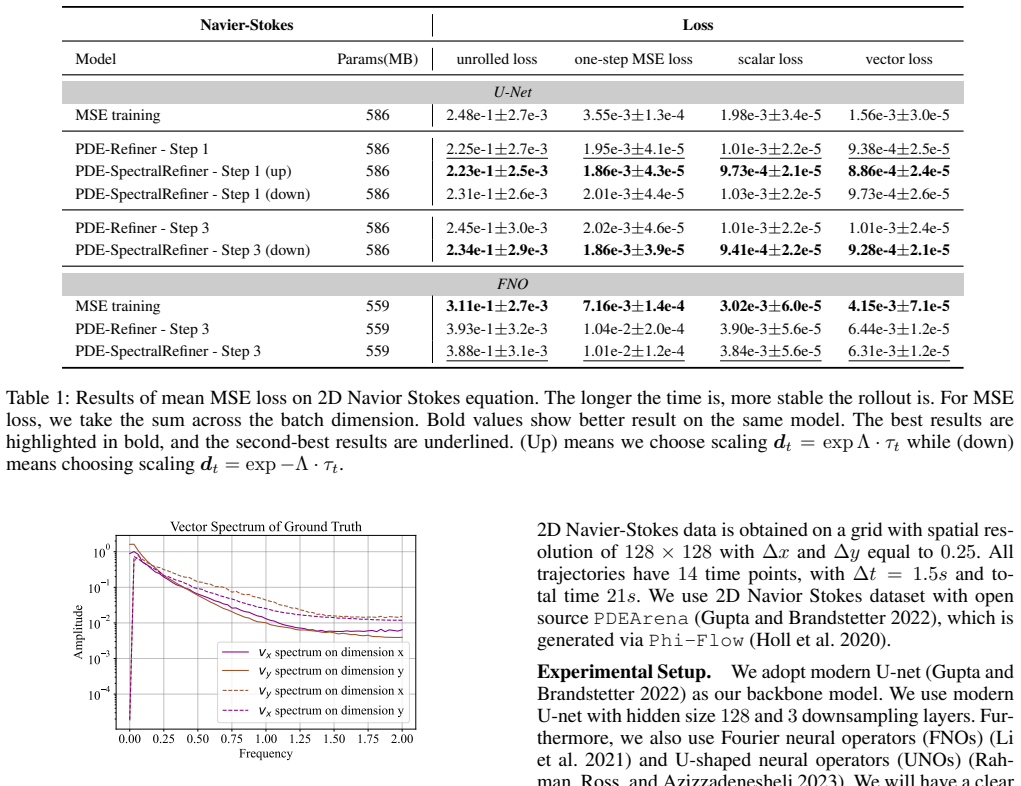
- With the down-scaling schedule $d_t=\exp(-\Lambda\tau_t)$, the model matches the high-frequency spectrum of 2D Navier-Stokes better than DDPM refinement and gives the best three-step refinement results on the U-Net backbone.
- With the up-scaling schedule $d_t=\exp(\Lambda\tau_t)$, the model concentrates on high frequencies immediately, which is the better one-step choice when only a single refinement step is available.
- For Fourier neural operators, where refinement with DDPM hurts accuracy, spectral adjustment partially recovers the loss; the paper attributes this to preserving signal-to-noise ratio and frequency-mode interactions under mode cutoff.
- The blurring schedule becomes a per-problem design parameter: the same framework can use different $\Lambda$ for different physical quantities whose spectra differ.
- Spectral reweighting changes only the amplitudes of the complex Fourier modes, not their phases, so it emphasizes frequencies without distorting their alignment.
Reading between the lines
- If the derivative identity in Eq. 14 holds generally, the blurring v-prediction should extend to other frequency schedules beyond the $\cos^2$ and $\sin^2$ cases the paper discusses, giving a family of refiners indexed by a spectral mask.
- The paper's own FNO results suggest a limit: refining already hurts Fourier operators with mode cutoff because noise breaks inter-frequency interactions; a natural testable extension is to mask noise only on high-frequency modes that the operator keeps, rather than the full spectrum.
- Because the claimed MSE recovery depends on a boundary calculation deferred to an appendix, a reader can settle the paper's core mechanism by differentiating $r_t^2$ directly before committing to the method.
- The anisotropic spectra of $v_x$ and $v_y$ in the Navier-Stokes data point toward direction-dependent blurring schedules as an obvious next test.
Editorial analysis
A structured set of objections, weighed in public.
Referee Report
Summary. The paper proposes PDESpectralRefiner, a modification of the diffusion-based PDE refiner PDERefiner in which the forward noise process is reweighted in Fourier space through a blurring schedule, so that different frequency components are corrupted at different rates. A new "blurring v-prediction" is introduced (Prop. 1, Eqs. 12–14) together with a corresponding sampling formula (Prop. 2, Eq. 15). The authors claim that with a cos^2 blurring schedule the first refinement step recovers the MSE objective, and they report improved one-step and rollout MSE for 2D Navier–Stokes with U-Net and FNO backbones.
Significance. The problem addressed—controlling high-frequency error accumulation in learned PDE surrogates—is important, and the idea of using blurring diffusion to reweight frequencies is a natural and potentially valuable extension of PDERefiner. The paper also makes a falsifiable methodological claim: the new v-prediction is the correct velocity for the spectrally reweighted process. I credit the authors for explicitly acknowledging limitations, including the poor FNO cooperation and the need for non-FFT projectors on non-uniform grids. However, the central derivation is not available in the submitted manuscript, the empirical gains are small and partly negative, and the experimental design has selection issues. If the derivation is corrected and the experiments are validated, the approach could be a useful tool, but in its current form the central claims are not verifiable.
major comments (3)
- [§4.1, Eq. (14)] The load-bearing identity for ∂r_t^2/∂φ_t is stated without proof, and the promised derivation is deferred to an appendix that is not present in the submitted manuscript. Prop. 1 (Eqs. 12–13) and Prop. 2 (Eq. 15) both depend on this identity, so no intermediate refinement step of the proposed method can be reproduced from the main text. Moreover, a direct calculation from Eqs. (10)–(11) with the standard blurring-diffusion parameterization α_t=cos φ, σ_t=sin φ, φ=πt/2 and the paper's proposed τ_t=(σ_B^2/2)cos^2 φ gives ∂r^2/∂φ = 2 sinφ cosφ [1 − exp(−σ_B^2 Λ cos^2 φ) + σ_B^2 Λ cos^2 φ exp(−σ_B^2 Λ cos^2 φ)], which does not match the structure of Eq. (14): the π/ln σ0 factor and the α^2/σ^2 · cos^3 sin prefactor are absent. The same mismatch occurs for the Hoogeboom sin^4 schedule. The authors need to supply the full derivation and state the exact α_t, σ_t, τ_t parameterization; otherwise the velocity used for training and sampling is not defined.
- [§4.1, "Resuming MSE training objective"] The t=1 boundary argument does not validate Eq. (14). At t=1, α_1=0 and σ_1=1 force the first term in Eq. (12) to −u_x for any schedule with τ_1=0, while the radial term in Eq. (13) vanishes only if the unverified condition ∂r_1^2/∂φ_1=0 holds. Thus the reported one-step MSE recovery is the standard DDPM v-prediction property and provides no evidence for the correctness of the new radial term at intermediate times. A numerical check of ∂r^2/∂φ against automatic differentiation, or an ablation that removes the radial term, is needed before the method can be considered validated.
- [§5.1, Table 1] The empirical support is weak and partially negative. On U-Net, the best relative gains over PDE-Refiner are about 4–5% (one-step MSE 1.86e-3 vs 1.95e-3; unrolled loss 2.34e-1 vs 2.45e-1 for step 3), with no significance testing and no ablation that isolates the effect of the blurring schedule from other changes. For FNO, both refinement approaches degrade performance relative to plain MSE training (3.88e-1 vs 3.11e-1), and the paper itself concedes poor FNO cooperation; the abstract's claim that PDESpectralRefiner is "more accurate for both one-step MSE loss and rollout loss" is therefore not supported in the FNO case. In addition, the blurring direction and maximum blur σ_B appear to be selected after inspecting the DDPM refiner's spectral errors; a validation-based selection protocol is needed to avoid overfitting the test set.
minor comments (6)
- [§3.3–§4] The notation α_t is heavily overloaded: Eq. (10)–(11) write α_t = α_t · d_t using the same symbol for the scaled and unscaled coefficients; introduce a distinct symbol such as \bar α_t for the scaled coefficient throughout.
- [§3.3–§4] The d_min term in the definition d_t = (1−d_min)exp(−Λτ_t)+d_min is silently dropped in §4's d_t = exp(−Λτ_t); the relationship between these definitions and the role of d_min should be stated explicitly.
- [Figures 2 and 3] The frequency-spectrum plots are essential to the motivation and analysis, but in the submitted text they appear as unreadable glyphs rather than legible figures; they should be regenerated and embedded correctly.
- [Throughout] There are numerous typos and terminological inconsistencies, including "Navior Stokes" for "Navier–Stokes", "stabling rollout" for "stable rollout", and "resume MSE training objective" where "recover" seems intended; the manuscript needs careful proofreading.
- [§4, Prop. 2 / Eq. (15)] The sampling formula in Eq. (15) should clarify whether u_x denotes the Fourier-transformed field and whether all operations are elementwise in spectral space; the text alternates between u_s and u_x for the same quantity, which is confusing.
- [§5.1, Table 1] The terms "Step 1" and "Step 3" and the relation of the first refinement step to the diffusion timestep t=1 should be defined precisely in the main text, since the interpretation of the reported losses depends on this convention.
Circularity Check
No significant circularity: the central v-prediction derivation is not fitted to the data, and the only by-construction element is the first-step MSE recovery, which is non-load-bearing for the reported rollout gains.
-
self definitional
[Section 4.1, 'Resuming MSE training objective' (after Proposition 1, Eqs. 12-14)]
"We can verify that, although the Equation 12 is quite intricate, this formula can also recover MSE training, with particular blurring schedule τt = σ2B/2 cos2(πt/2), r1 = 1 and ∂r2t/∂ϕt = −2αt × 0 × ... = 0, we have v1 = 1/1 · (0 · exp(−Λ · τt)uϵ − 1ux) + 0 = −ux."
The claimed 'recovering MSE training objective' is obtained by choosing the blurring schedule so that at t=1 one has α1=0, σ1=1, r1=1 and ∂r2/∂ϕ=0; substituting these endpoint values into Eq. 12 gives v1=-ux. The property is therefore equivalent to the boundary conditions used to define the schedule, not an independent consequence of the new radial term in Eq. 14. The paper presents this as a contribution, but it is a design constraint. It is not load-bearing for the main empirical claim, because the reported NS improvements are attributed to intermediate refinement steps where the radial term is active; hence this is a minor self-definitional element rather than a central circularity.
full rationale
Prop. 1 (Eqs. 12-14) is presented as a derivation from the blurring diffusion forward process; it is not fitted to the NS data or to the MSE objective. The only self-definitional element is the 'Resuming MSE training objective' claim: the schedule τt = σB^2/2 cos^2(πt/2) is chosen so that α1=0, σ1=1, r1=1 and ∂r2/∂ϕ=0, which forces v1=-ux. This makes the first-step MSE recovery an endpoint condition rather than an independent consequence of the new radial term; it is not load-bearing for the reported rollout gains, which depend on intermediate refinement steps. The choice of blurring direction and maximum blur is reported as a hyperparameter sweep over [2,4,8]/[2,4], not as a fitted parameter disguised as a prediction. The main weakness is not circularity: Eq. 14's derivative is deferred to an appendix that is absent, and Prop. 2 inherits this unverified identity. That is a completeness/correctness problem, not a circular reduction. I therefore score 2 for the minor by-construction MSE-recovery contribution.
Assumptions & free parameters
free parameters (3)
- maximum blur sigma_B =
2, 4, or 8 (per schedule, chosen by validation)
- blurring direction =
exp(+Lambda*tau) (up) or exp(-Lambda*tau) (down), chosen per dataset
- scaling/shape of Lambda =
not specified exactly; follows frequency-squared sum in the experiments
assumptions (4)
- domain assumption The blurring diffusion forward process q(u_t|u_s) with u_t = d_t alpha_t u_s + sigma_t epsilon and variance-preserving noise is a valid generative process.
- ad hoc to paper The derivative d r_t^2 / d phi_t in Eq. 14 is correct as stated.
- ad hoc to paper With tau_t = (sigma_B^2/2)cos^2(pi t/2), at t=1 one has r_1=1 and d r_1^2 / d phi_1 = 0, giving v_1 = -u_x.
- domain assumption The 2D Navier-Stokes data has an energy cascade with more high-frequency energy than KS, so the spectral mismatch justifies the new schedule.
Cite this review
Pith. "Pith review of PDESpectralRefiner: Achieving More Accurate Long Rollouts with Spectral Adjustment." pith.science (2026). https://pith.science/paper/3BEBMHIN
@misc{pith2026250610711,
  author       = {Pith},
  title        = {Pith review of: PDESpectralRefiner: Achieving More Accurate Long Rollouts with Spectral Adjustment},
  year         = {2026},
  howpublished = {\url{https://pith.science/paper/3BEBMHIN}},
  note         = {Machine review of arXiv:2506.10711}
}
read the original abstract
Generating accurate and stable long rollouts is a notorious challenge for time-dependent PDEs (Partial Differential Equations). Recently, motivated by the importance of high-frequency accuracy, a refiner model called PDERefiner utilizes diffusion models to refine outputs for every time step, since the denoising process could increase the correctness of modeling high frequency part. For 1-D Kuramoto-Sivashinsky equation, refiner models can degrade the amplitude of high frequency part better than not doing refinement process. However, for some other cases, the spectrum might be more complicated. For example, for a harder PDE like Navior-Stokes equation, diffusion models could over-degrade the higher frequency part. This motivates us to release the constraint that each frequency weighs the same. We enhance our refiner model with doing adjustments on spectral space, which recovers Blurring diffusion models. We developed a new v-prediction technique for Blurring diffusion models, recovering the MSE training objective on the first refinement step. We show that in this case, for different model backbones, such as U-Net and neural operators, the outputs of PDE-SpectralRefiner are more accurate for both one-step MSE loss and rollout loss.
Figures


Reference graph
Works this paper leans on
-
[1]
The Kuramoto-Sivashinsky Equation
Baez, J. C.; Huntsman, S.; and Weis, C. 2022. The Kuramoto--Sivashinky Equation. arXiv preprint arXiv:2210.01711
work page Pith review arXiv 2022
-
[2]
Bao, F.; Li, C.; Zhu, J.; and Zhang, B. 2022. Analytic- DPM : an Analytic Estimate of the Optimal Reverse Variance in Diffusion Probabilistic Models. In International Conference on Learning Representations
work page 2022
-
[3]
Bao, F.; Zhao, M.; Hao, Z.; Li, P.; Li, C.; and Zhu, J. 2023. Equivariant Energy-Guided SDE for Inverse Molecular Design. In The Eleventh International Conference on Learning Representations
work page 2023
-
[4]
Brandstetter, J.; Worrall, D. E.; and Welling, M. 2022. Message Passing Neural PDE Solvers. In International Conference on Learning Representations
work page 2022
-
[5]
Dhariwal, P.; and Nichol, A. Q. 2021. Diffusion Models Beat GAN s on Image Synthesis. In Beygelzimer, A.; Dauphin, Y.; Liang, P.; and Vaughan, J. W., eds., Advances in Neural Information Processing Systems
work page 2021
-
[6]
Gupta, J. K.; and Brandstetter, J. 2022. Towards Multi-spatiotemporal-scale Generalized PDE Modeling. arXiv preprint arXiv:2209.15616
arXiv 2022
-
[7]
Ho, J.; Jain, A.; and Abbeel, P. 2020. Denoising diffusion probabilistic models. Advances in neural information processing systems, 33: 6840--6851
2020
-
[8]
Holl, P.; Koltun, V.; Um, K.; and Thuerey, N. 2020. phiflow: A differentiable pde solving framework for deep learning via physical simulations. In NeurIPS workshop, volume 2
work page 2020
Show all 32 references
-
[9]
Hoogeboom, E.; and Salimans, T. 2023. Blurring Diffusion Models. In The Eleventh International Conference on Learning Representations
2023
-
[10]
G.; Vignac, C.; and Welling, M
Hoogeboom, E.; Satorras, V. G.; Vignac, C.; and Welling, M. 2022. Equivariant diffusion for molecule generation in 3d. In International conference on machine learning, 8867--8887. PMLR
2022
-
[11]
Jing, B.; Corso, G.; Chang, J.; Barzilay, R.; and Jaakkola, T. 2022. Torsional diffusion for molecular conformer generation. Advances in Neural Information Processing Systems, 35: 24240--24253
2022
-
[12]
B.; Azizzadenesheli, K.; liu, B.; Bhattacharya, K.; Stuart, A.; and Anandkumar, A
Li, Z.; Kovachki, N. B.; Azizzadenesheli, K.; liu, B.; Bhattacharya, K.; Stuart, A.; and Anandkumar, A. 2021. Fourier Neural Operator for Parametric Partial Differential Equations. In International Conference on Learning Representations
2021
-
[13]
Lippe, P.; Veeling, B.; Perdikaris, P.; Turner, R.; and Brandstetter, J. 2024. Pde-refiner: Achieving accurate long rollouts with neural pde solvers. Advances in Neural Information Processing Systems, 36
2024
-
[14]
Q.; and Dhariwal, P
Nichol, A. Q.; and Dhariwal, P. 2021. Improved denoising diffusion probabilistic models. In International conference on machine learning, 8162--8171. PMLR
2021
-
[15]
Pfaff, T.; Fortunato, M.; Sanchez-Gonzalez, A.; and Battaglia, P. 2021. Learning Mesh-Based Simulation with Graph Networks. In International Conference on Learning Representations
2021
-
[16]
A.; Ross, Z
Rahman, M. A.; Ross, Z. E.; and Azizzadenesheli, K. 2023. U- NO : U-shaped Neural Operators. Transactions on Machine Learning Research
2023
-
[17]
Ramesh, A.; Dhariwal, P.; Nichol, A.; Chu, C.; and Chen, M. 2022. Hierarchical text-conditional image generation with clip latents. arXiv preprint arXiv:2204.06125, 1(2): 3
2022 arXiv
-
[18]
Rissanen, S.; Heinonen, M.; and Solin, A. 2023. Generative Modelling with Inverse Heat Dissipation. In The Eleventh International Conference on Learning Representations
2023
-
[19]
Salimans, T.; and Ho, J. 2022. Progressive Distillation for Fast Sampling of Diffusion Models. In International Conference on Learning Representations
2022
-
[20]
Sanchez-Gonzalez, A.; Godwin, J.; Pfaff, T.; Ying, R.; Leskovec, J.; and Battaglia, P. W. 2020. Learning to Simulate Complex Physics with Graph Networks. In International Conference on Machine Learning
2020
-
[21]
Sohl-Dickstein, J.; Weiss, E.; Maheswaranathan, N.; and Ganguli, S. 2015. Deep unsupervised learning using nonequilibrium thermodynamics. In International conference on machine learning, 2256--2265. PMLR
2015
-
[22]
Song, J.; Meng, C.; and Ermon, S. 2021. Denoising Diffusion Implicit Models. In International Conference on Learning Representations
2021
-
[23]
Song, Y.; and Ermon, S. 2019. Generative modeling by estimating gradients of the data distribution. Advances in neural information processing systems, 32
2019
-
[24]
P.; Kumar, A.; Ermon, S.; and Poole, B
Song, Y.; Sohl-Dickstein, J.; Kingma, D. P.; Kumar, A.; Ermon, S.; and Poole, B. 2021. Score-Based Generative Modeling through Stochastic Differential Equations. In International Conference on Learning Representations
2021
-
[25]
Temam, R. 2001. Navier-Stokes equations: theory and numerical analysis, volume 343. American Mathematical Soc
2001
-
[26]
W.; and Holmes, P
Wittenberg, R. W.; and Holmes, P. 1999. Scale and space localization in the Kuramoto--Sivashinsky equation. Chaos: An Interdisciplinary Journal of Nonlinear Science, 9(2): 452--465
1999
-
[27]
Wu, T.; Maruyama, T.; Wei, L.; Zhang, T.; Du, Y.; Iaccarino, G.; and Leskovec, J. 2024. Compositional Generative Inverse Design. In The Twelfth International Conference on Learning Representations
2024
-
[28]
Wu, T.; Maruyama, T.; Zhao, Q.; Wetzstein, G.; and Leskovec, J. 2023. Learning Controllable Adaptive Simulation for Multi-resolution Physics. In The Eleventh International Conference on Learning Representations
2023
-
[29]
Xu, M.; Yu, L.; Song, Y.; Shi, C.; Ermon, S.; and Tang, J. 2022. GeoDiff: A Geometric Diffusion Model for Molecular Conformation Generation. In International Conference on Learning Representations
2022
-
[30]
Zhang, X.; Wang, L.; Helwig, J.; Luo, Y.; Fu, C.; Xie, Y.; Liu, M.; Lin, Y.; Xu, Z.; Yan, K.; et al. 2023. Artificial intelligence for science in quantum, atomistic, and continuum systems. arXiv preprint arXiv:2307.08423
2023 arXiv
-
[31]
, " * write output.state after.block = add.period write newline
ENTRY address archivePrefix author booktitle chapter edition editor eid eprint howpublished institution isbn journal key month note number organization pages publisher school series title type volume year label extra.label sort.label short.list INTEGERS output.state before.all...
-
[32]
write newline
" write newline "" before.all 'output.state := FUNCTION n.dashify 't := "" t empty not t #1 #1 substring "-" = t #1 #2 substring "--" = not "--" * t #2 global.max substring 't := t #1 #1 substring "-" = "-" * t #2 global.max substring 't := while if t #1 #1 substring * t #2 gl...
Reviewed August 7, 2026 · model on record in the stance chip above.
Discussion (0). Sign in to comment.