REVIEW 3 major objections 4 minor 25 references
Scalable Learning of High-Dimensional Demonstrations with Composition of Linear Parameter Varying Dynamical Systems
T0 review · 3 major / 4 minor · reviewed 2026-08-06 · deepseek-v4-flash
Pith's one-line read The paper claims that splitting a high-dimensional dynamical-system learning problem into coupled subsystems makes the LPV-DS technique scale to 7D joint-space demonstrations, producing stable dynamical systems in a few minutes where the…
desk verdict Compositional LPV-DS learning is a good idea, but the main stability proof has fixable algebraic errors and the scaling claim needs more than two undocumented examples. read the letter →
The pith
A machine-rendered reading of the paper's core claim, the machinery that carries it, and where it could break.
The reading
What carries the argument
The central object is the interconnection of dynamical subsystems with an internal coupling matrix $M$, together with per-subsystem matrices $D_i$ appearing in the sub-Lyapunov dissipation inequalities. The argument turns on Theorem 1: if the block-diagonal matrix built from the weighted $D_i$ satisfies the quadratic inequality (10) with the stacked matrix $[M; I]$, then the weighted sum of sub-Lyapunov functions is a genuine Lyapunov function for the full system. Theorem 2 converts each subsystem's stability constraints into an LMI plus a BMI, so the subsystem-level optimization is numerically tractable, and the global composition step only has to find the weights $\mu_i$.
What would settle it
Construct a 7D demonstration whose optimal DS has a scheduling function that depends on a combination of two joints, run the proposed algorithm with the per-joint decomposition used in Example 1, and check whether the learned DS tracks the demonstrations and remains stable; if it cannot match the accuracy of a monolithic solver on data the monolithic solver can handle, the local-scheduling and hand-chosen-$M$ assumptions are the point of failure.
Extended reading notes
Core claim
The central claim is that a stable high-dimensional LPV-DS can be learned by composition: split the state into $N$ subsystems, solve a small LPV-DS learning problem for each subsystem with its own quadratic sub-Lyapunov function, and then combine the pieces by finding nonnegative weights $\mu_i$ that satisfy a coupling inequality. Theorem 1 states that under that inequality the weighted sum $V(x)=\sum_{i=1}^N \mu_i V_i(x_i)$ is a Lyapunov function for the interconnected system, and Theorem 2 shows that when each subsystem's dynamics are LPV with scheduling functions that depend only on the local state, the per-subsystem constraints become a linear matrix inequality plus a bilinear matrix inequality that numerical solvers can handle. The paper reports learning times around 100–150 seconds for 7D joint-space examples where the monolithic LPV-DS solver fails to converge, along with simulations and real-robot tracking that match the demonstrations.
Load-bearing premise
The scheduling functions $\gamma_k$ in each subsystem depend only on that subsystem's own state $x_i$, not on the full state, and the interconnection matrix $M$ is chosen by hand for each task, so the method's success depends on a favorable decomposition and there is no bound on the error introduced by the local-scheduling restriction.
Editorial extensions
If this is right
- The compositional approach learns stable 7D joint-space dynamical systems in roughly 100–150 seconds, where the monolithic LPV-DS solver fails to converge.
- Learning directly in joint space avoids inverse-kinematics approximations and can reproduce end-effector orientation changes, as shown in Experiment 1.
- The interconnection structure can be chosen flexibly rather than fully connected, and the resulting DS remains stable and accurate, as in Example 2.
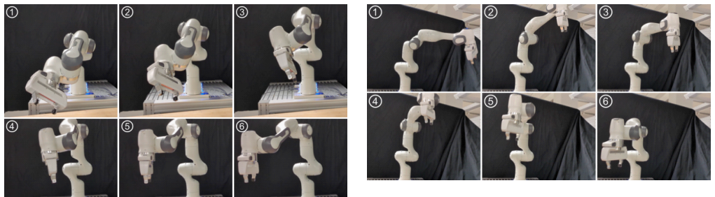
- A real robot with a joint impedance controller can track trajectories generated by the learned DS, so the method transfers from simulation to hardware.
- The framework's run time stays on the order of minutes on a laptop, which makes repeated re-learning of tasks practical.
Reading between the lines
- Because Theorem 1 is stated for the generic stable-DS optimization (2), the same composition argument may transfer to other BMI-based stable-DS learners, such as polynomial or barrier-certified variants, not just LPV-DS.
- The local-scheduling restriction suggests a natural stress test: tasks where a joint's correct motion depends on another joint's configuration may be under-approximated, and allowing the scheduling function to depend on a small learned subset of the full state could widen the representable class.
- A data-driven choice of the interconnection matrix $M$, based on measured cross-dimensional correlations in the demonstrations, could remove the current hand-design step and make the method more automatic.
Signed reviews
Editorial analysis
A structured set of objections, weighed in public.
Referee Report
Summary. The paper proposes a compositional framework to scale linear parameter-varying dynamical system (LPV-DS) learning to high-dimensional demonstrations, such as 7-DOF joint-space trajectories. The method decomposes the full DS into smaller subsystems, solves a subsystem-level optimization subject to LMI/BMI constraints (Theorem 2), and then composes the subsystems via dissipativity theory, certifying global stability through a weighted sum of sub-Lyapunov functions (Theorem 1). Experiments on simulated 7-DOF joint-space data and a real Franka Emika robot show that the approach learns stable DSs in minutes where the vanilla LPV-DS solver fails, and it achieves lower error than or comparable error to the neural SNDS baseline in the tested tasks.
Significance. If correct, this is a valuable contribution to LfD for high-dimensional joint-space tasks. The paper builds on established dissipativity theory rather than a self-referential stability condition, and it validates the approach with both simulation and hardware experiments, reporting concrete runtimes and comparisons. The compositional strategy is a plausible way to alleviate the non-convex BMI bottleneck, and the reported results support the narrative that the method scales where the vanilla technique does not. However, the formal stability guarantee in Theorem 1 is not established as written, because the proof in Appendix I drops the weights μ_i and defines the decay constant incorrectly. The paper also restricts the scheduling functions to local state without quantifying the induced representational limitation. These issues need to be resolved before the central scaling claim can be fully accepted.
major comments (3)
- [Appendix I, proof of Theorem 1 (also Theorem 1 statement and Eq. (12))] The proof of condition (2c) is invalid as written. The theorem defines V(x) = Σ_i μ_i V_i(x_i), but the bounding step sums the unweighted inequalities (9c) to obtain δ = N min_i δ_i and δ̄ = N max_i δ̄_i, with no μ_i appearing. This can only hold if all μ_i equal 1. Additionally, the derivative bound defines ξ := min_i μ_i ξ_i, but concluding V̇(x) ≤ −ξV(x) from V̇(x) ≤ −Σ_i μ_i ξ_i V_i(x_i) requires μ_i ξ_i ≥ ξ μ_i for every i with μ_i > 0, i.e., ξ_i ≥ ξ; the printed definition only guarantees μ_i ξ_i ≥ ξ, which does not imply the needed inequality. Finally, Theorem 1 assumes μ_i ≥ 0, yet if any μ_i = 0, the weighted sum V(x) is not positive definite in that coordinate, so it cannot certify stability of the full interconnected state. These are not cosmetic issues: Theorem 1 is the only formal bridge from the subsystem conditions to the global stability guarantee of Algorithm 1. Please correct the proof, e.g., by requiring μ_i > 0 and defining δ = min_i μ_i δ_i, δ̄ = max_i μ_i δ̄_i, ξ = min_i ξ_i, or by providing an equivalent correct argument.
- [Section III, Eq. (13) and Section IV] The scheduling functions γ_k in the subsystem dynamics (13) depend only on the local state x_i, whereas the original LPV-DS formulation in Eq. (5) uses γ_k(x) depending on the full state. This restricts the class of representable DSs: the modulation of local dynamics cannot depend on remote joint states. The paper does not quantify the approximation error induced by this restriction, nor does it discuss which tasks are faithfully representable. Because the paper claims to 'scale the LPV-DS technique' to high-dimensional demonstrations, this local-scheduling restriction should be explicitly stated as a modeling limitation and, ideally, accompanied by an error analysis or a discussion of the class of demonstrations for which it is adequate.
- [Section IV, Examples 1 and 2, and Remark 3] The interconnection matrix M is hand-designed for each example, and Remark 3 acknowledges that no automated selection criterion is provided. The success of the compositional method depends on choosing a favorable decomposition, and the paper does not offer guidance on how to select M for a new task or how suboptimal choices affect the existence of μ_i satisfying condition (10). This is not a correctness error, but it limits the generality of the claimed scalability and should be discussed more explicitly as an open problem, perhaps with a sensitivity study on M.
minor comments (4)
- [Notation, Section II] The notation line 'R>0, R≥0 and N' is not typeset correctly; it should read 'R_{>0}, R_{\ge 0}' and '\mathbb{N}' for the positive reals, nonnegative reals, and positive integers, respectively.
- [Throughout] There are multiple typographical issues, such as missing superscripts in the objective functions (e.g., 'PM k=1' instead of '\sum_{k=1}^M') and the phrase 'author’s knowledge' should be 'authors’ knowledge'.
- [Table I and experimental sections] The table would benefit from a column header indicating that 'Run Time' is in seconds and from a note on the hardware used; the text in Sections IV and V already gives this information, but a concise table caption would improve readability.
- [Section V] In the experimental description, the controller is described as a 'joint impedance controller' used with the joint velocity interface; briefly clarifying how the DS output is converted to torque or velocity commands would help reproducibility.
Circularity Check
No circularity found: the compositional stability guarantee is inherited from an external dissipativity theorem and a separate feasibility step, not from the fitted parameters; a proof bug in Theorem 1 is a correctness issue rather than circular reasoning.
full rationale
The paper's derivation chain is not circular. The scheduling functions γ_k are obtained from the demonstration data via the GMM procedure of [9] (Figueroa and Billard, not the present authors), and the subsystem matrices A_ki, B_ki are fitted subject to the local LMIs/BMI (14)-(15). Stability is then certified in a separate step: the multipliers μ_i are found by solving the quadratic inequality (10), and the candidate Lyapunov function V(x)=Σμ_iV_i(x_i) is justified through the external dissipativity result [21] (Arcak, Meissen, Packard). The μ_i are not functions of A_ki or B_ki and inequality (10) is independent of the fitted outputs, so the stability claim is not an encoding of the fit. The claim that f minimizes (2a) follows from the decomposition identity in Appendix I, which is an algebraic equality, not a tautology. The experiments use an external Franka controller and compare against SNDS [20], providing external falsifiability. The citations to [15] (which shares authors) are for the demonstration dataset and are not load-bearing; no uniqueness theorem from the same authors is invoked. I do flag a separate, non-circular correctness defect in the proof of Theorem 1: in Appendix I the coordinate bound on V(x) is obtained by summing (9c) without the weights μ_i ('Applying summation to both sides of the inequality (9c) ... one can draw the conclusion that Σδ_i‖x_i‖² ≤ ΣV_i(x_i) ≤ Σδ̄_i‖x_i‖², which can be rewritten as δ‖x‖² ≤ V(x) ≤ δ̄‖x‖²'), and the final line defines ξ := min_i μ_iξ_i although the required inequality is V̇≤−ξV with ξ≤ξ_i; also μ_i>0 is not assumed, so V may fail positive definiteness. This invalidates the printed proof but is not circularity: the theorem is not made true by its own assumptions by construction. Score 0 for circularity.
Assumptions & free parameters
free parameters (3)
- Number of GMM components K per subsystem
- Dissipativity constants delta_i, delta_i_bar, xi_i
- Interconnection matrix M =
hand-designed per example
assumptions (4)
- domain assumption Compositional dissipativity certification conditions from Arcak et al. are valid for the constructed interconnection
- domain assumption The numerical solvers PENLAB/YALMIP return feasible solutions for the BMIs and LMIs
- domain assumption Demonstration data has a unique equilibrium at the origin and distinct points
- standard math GMM scheduling functions gamma_k sum to one and are positive
Cite this review
Pith. "Pith review of Scalable Learning of High-Dimensional Demonstrations with Composition of Linear Parameter Varying Dynamical Systems." pith.science (2026). https://pith.science/paper/CBGWTQNY
@misc{pith2026250703992,
  author       = {Pith},
  title        = {Pith review of: Scalable Learning of High-Dimensional Demonstrations with Composition of Linear Parameter Varying Dynamical Systems},
  year         = {2026},
  howpublished = {\url{https://pith.science/paper/CBGWTQNY}},
  note         = {Machine review of arXiv:2507.03992}
}
read the original abstract
Learning from Demonstration (LfD) techniques enable robots to learn and generalize tasks from user demonstrations, eliminating the need for coding expertise among end-users. One established technique to implement LfD in robots is to encode demonstrations in a stable Dynamical System (DS). However, finding a stable dynamical system entails solving an optimization problem with bilinear matrix inequality (BMI) constraints, a non-convex problem which, depending on the number of scalar constraints and variables, demands significant computational resources and is susceptible to numerical issues such as floating-point errors. To address these challenges, we propose a novel compositional approach that enhances the applicability and scalability of learning stable DSs with BMIs.
Figures


Figures from the paper (3 more)


Reference graph
Works this paper leans on
-
[1]
A. Billard, S. Calinon, R. Dillmann, and S. Schaal, Robot Pro- gramming by Demonstration . Berlin, Heidelberg: Springer Berlin Heidelberg, 2008, pp. 1371–1394
work page 2008
-
[2]
A survey of robot learning from demonstration,
B. Argall, S. Chernova, M. Veloso, and B. Browning, “A survey of robot learning from demonstration,” Robotics and Autonomous Systems, vol. 57, pp. 469–483, 05 2009
work page 2009
-
[3]
Recent advances in robot learning from demonstration,
H. Ravichandar, A. S. Polydoros, S. Chernova, and A. Billard, “Recent advances in robot learning from demonstration,” Annual review of control, robotics, and autonomous systems , vol. 3, no. 1, pp. 297– 330, 2020
work page 2020
-
[4]
A. Billard, S. Mirrazavi, and N. Figueroa, Learning for Adaptive and Reactive Robot Control: A Dynamical Systems Approach. MIT Press, 2022
work page 2022
-
[5]
Y . Shavit, N. Figueroa, S. S. M. Salehian, and A. Billard, “Learning augmented joint-space task-oriented dynamical systems: a linear pa- rameter varying and synergetic control approach,” IEEE Robotics and Automation Letters, vol. 3, no. 3, pp. 2718–2725, 2018
work page 2018
-
[6]
Orientation in Carte- sian space dynamic movement primitives,
A. Ude, B. Nemec, T. Petri ´c, and J. Morimoto, “Orientation in Carte- sian space dynamic movement primitives,” in 2014 IEEE International Conference on Robotics and Automation (ICRA) . IEEE, 2014, pp. 2997–3004
work page 2014
-
[7]
Gaussian mixture model for 3-dof orientations,
S. Kim, R. Haschke, and H. Ritter, “Gaussian mixture model for 3-dof orientations,” Robotics and Autonomous Systems , vol. 87, pp. 28–37, 2017
work page 2017
-
[8]
An approach for imitation learning on Riemannian manifolds,
M. J. A. Zeestraten, I. Havoutis, J. a. Silv ´erio, S. Calinon, and D. G. Caldwell, “An approach for imitation learning on Riemannian manifolds,” IEEE Robotics and Automation Letters , vol. 2, no. 3, pp. 1240–1247, 2017
work page 2017
Show all 25 references
-
[9]
A physically-consistent Bayesian non- parametric mixture model for dynamical system learning,
N. Figueroa and A. Billard, “A physically-consistent Bayesian non- parametric mixture model for dynamical system learning,” in Confer- ence on Robot Learning . PMLR, 2018, pp. 927–946
2018
-
[10]
Locally active globally stable dynamical systems: theory, learning, and experiments,
——, “Locally active globally stable dynamical systems: theory, learning, and experiments,” The International Journal of Robotics Research, vol. 41, no. 3, pp. 312–347, 2022
2022
-
[11]
On the NP-hardness of solving bilinear matrix inequalities and simultaneous stabilization with static output feedback,
O. Toker and H. Ozbay, “On the NP-hardness of solving bilinear matrix inequalities and simultaneous stabilization with static output feedback,” in Proceedings of 1995 American Control Conference , vol. 4. IEEE, 1995, pp. 2525–2526
1995
-
[12]
Branch-and-cut algorithms for the bilinear matrix inequality eigenvalue problem,
M. Fukuda and M. Kojima, “Branch-and-cut algorithms for the bilinear matrix inequality eigenvalue problem,” Computational Optimization and Applications, vol. 19, pp. 79–105, 2001
2001
-
[13]
Validating nu- merical semidefinite programming solvers for polynomial invariants,
P. Roux, Y .-L. V oronin, and S. Sankaranarayanan, “Validating nu- merical semidefinite programming solvers for polynomial invariants,” Formal Methods in System Design , vol. 53, pp. 286–312, 2018
2018
-
[14]
Learning Lyapunov-stable polynomial dynamical systems through imitation,
A. Abyaneh and H.-C. Lin, “Learning Lyapunov-stable polynomial dynamical systems through imitation,” in Proceedings of the 2023 Conference on Robot Learning (CoRL 2023) , 2023
2023
-
[15]
Learning barrier-certified polynomial dynamical systems for obstacle avoidance with robots,
M. Schonger, H. T. Kussaba, L. Chen, L. Figueredo, A. Swikir, A. Billard, and S. Haddadin, “Learning barrier-certified polynomial dynamical systems for obstacle avoidance with robots,” in Proceedings of the 2024 International Conference on Robotics and Automation , 2024, pp. 1...
2024
-
[16]
Learning stable nonlinear dynamical systems with Gaussian mixture models,
S. M. Khansari-Zadeh and A. Billard, “Learning stable nonlinear dynamical systems with Gaussian mixture models,” IEEE Transactions on Robotics, vol. 27, no. 5, pp. 943–957, Oct. 2011
2011
-
[17]
Learning stable deep dynamics models,
J. Z. Kolter and G. Manek, “Learning stable deep dynamics models,” Advances in neural information processing systems , vol. 32, 2019
2019
-
[18]
Euclideanizing flows: Diffeomorphic reduction for learning stable dynamical systems,
M. A. Rana, A. Li, D. Fox, B. Boots, F. Ramos, and N. Ratliff, “Euclideanizing flows: Diffeomorphic reduction for learning stable dynamical systems,” in Learning for Dynamics and Control . PMLR, 2020, pp. 630–639
2020
-
[19]
Almost surely stable deep dynamics,
N. Lawrence, P. Loewen, M. Forbes, J. Backstrom, and B. Gopaluni, “Almost surely stable deep dynamics,”Advances in Neural Information Processing Systems, vol. 33, pp. 18 942–18 953, 2020
2020
-
[20]
Globally stable neural im- itation policies,
A. Abyaneh, M. S. Guzm ´an, and H.-C. Lin, “Globally stable neural im- itation policies,” in 2024 IEEE International Conference on Robotics and Automation (ICRA) . IEEE, 2024, pp. 15 061–15 067
2024
-
[21]
Arcak, C
M. Arcak, C. Meissen, and A. Packard, Networks of dissipative systems: compositional certification of stability, performance, and safety. Springer, 2016
2016
-
[22]
PENLAB: A MATLAB solver for nonlinear semidefinite optimization,
J. Fiala, M. Ko ˇcvara, and M. Stingl, “PENLAB: A MATLAB solver for nonlinear semidefinite optimization,” 2013. [Online]. Available: https://arxiv.org/abs/1311.5240
2013 arXiv
-
[23]
Compliant control of uni/multi-robotic arms with dynamical systems,
S. S. M. Salehian, “Compliant control of uni/multi-robotic arms with dynamical systems,” EPFL, Technical report, 2018
2018
-
[24]
Y ALMIP: A toolbox for modeling and optimization in MATLAB,
J. L ¨ofberg, “Y ALMIP: A toolbox for modeling and optimization in MATLAB,” in 2004 IEEE international conference on robotics and automation. IEEE, 2004, pp. 284–289
2004
-
[25]
The Franka Emika robot: A reference platform for robotics research and education,
S. Haddadin, S. Parusel, L. Johannsmeier, S. Golz, S. Gabl, F. Walch, M. Sabaghian, C. Jaehne, L. Hausperger, and S. Haddadin, “The Franka Emika robot: A reference platform for robotics research and education,” IEEE Robotics & Automation Magazine , 2022
2022
Reviewed August 6, 2026 · model on record in the stance chip above.
Discussion (0). Continue with ORCID to comment.