REVIEW 3 major objections 5 minor 47 references
A Tax-Efficient Model Predictive Control Policy for Retirement Funding
T0 review · 3 major / 5 minor · reviewed 2026-08-06 · deepseek-v4-flash
Pith's one-line read Solving a convex optimization problem each year to re-plan withdrawals and Roth conversions funds a fixed inflation-adjusted consumption while leaving a larger bequest than the 4% rule in about 70% of simulated retirements.
desk verdict Solid convex-MPC formulation for retirement funding, but the claimed edge over the 4% rule rests on a weak proportional-withdrawal benchmark, not a fair tax-aware comparison. read the letter →
The pith
A machine-rendered reading of the paper's core claim, the machinery that carries it, and where it could break.
The reading
What carries the argument
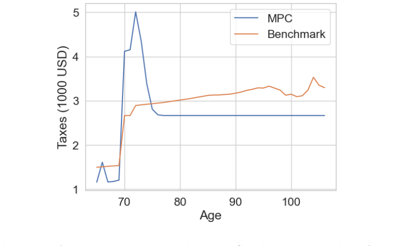
The engine of the paper is the retirement funding planning (RFP) problem, a convex optimization problem with roughly $13T$ variables for a $T$-year horizon that selects withdrawals, deposits, and Roth conversions across brokerage, IRA, and Roth accounts. Its convexity comes from relaxing the tax constraint $\tau_t = \phi(\omega_t) + \xi(b_t)_+(1-\delta_0)_+$ to an inequality $\tau_t \ge \phi(\omega_t) + \xi(b_t)_+(1-\delta_0)$, since overpaying taxes can never improve the objective and the relaxation is tight at the optimum. The second moving part is the annual update-plan-act loop: each year the retiree solves the RFP with current account values, a planning horizon set to 150% of remaining life expectancy, and current forecasts, then executes only the first year's actions. In the simulations the policy's signature behavior is aggressive Roth conversion in the early retirement years, while the retiree is in a lower tax bracket, followed by tax-free Roth growth that funds the larger bequest.
What would settle it
Run the same MPC-versus-benchmark comparison out-of-sample: fit the Gaussian mixture and VAR models only on data through 1990, generate trajectories with the realized 1991-2023 returns and inflation, and check whether the relative bequest still centers near 1.06 with the MPC policy better in about 70% of cases. A cleaner version is a pure historical backtest, replaying both policies on the actual 1962-2023 sequence and on block-bootstrap reorderings of it; if the bequest advantage shrinks toward zero or reverses, the claimed superiority is an artifact of the chosen statistical models rather than a property of the policy.
Extended reading notes
Core claim
The paper's central claim is that the retirement funding planning problem admits a convex formulation, and that wrapping this planner in a model predictive control loop yields a policy that dominates the standard 4% rule. The planner maximizes the bequest subject to a constant real consumption target; the key move is relaxing the tax-bill equality constraint to an inequality, justified because a retiree would never voluntarily pay more tax than required, so the relaxation is tight at any optimum. Solved annually with updated balances, life expectancy, and return forecasts, the planner's first-year actions become the policy. Across 1,000 simulated lifetimes for two typical US retirees, the policy delivers the target consumption in over 98% of scenarios and a bequest larger than the benchmark in about two-thirds to 70% of scenarios, with a median relative bequest of 1.06; when it beats the benchmark, the median increase is 12-14%.
Load-bearing premise
The evaluation treats statistical models fitted to historical data, a three-component Gaussian mixture for stock returns and a vector autoregression with a hand-chosen piecewise-linear transform for Treasury rates and inflation, as a faithful stand-in for future market behavior, so the simulated bequest advantage may not transfer to real retirement outcomes if the future deviates from the fitted distributions.
Editorial extensions
If this is right
- If the paper's simulations are representative, replacing a fixed withdrawal rule with the yearly re-planning policy preserves consumption in nearly all scenarios and increases the expected inheritance left to heirs, with a median bequest gain of about 6%.
- The policy's advantage traces to a specific mechanism, front-loaded Roth conversions, so retirees looking to copy the result should expect to convert IRA funds to Roth early, before taxable income rises at age 70.
- Because each planning problem solves in about 0.01 seconds, the policy is cheap enough to run on a laptop and to evaluate over thousands of scenarios before adoption.
- The same convex planner extends to 401(k) and Roth 401(k) accounts, five-year Roth rules, MAGI-dependent contribution limits, and collar-protected portfolios without changing the architecture.
- If the retiree uses collar options or conservative return forecasts in the planner, worst-case bequest outcomes tighten while the median outcome is largely unchanged, so the policy can be tuned for risk aversion.
Reading between the lines
- Beyond the paper: a natural stress test the authors do not run is to fit the return and inflation models on a pre-1990 window and evaluate the policy on the post-1990 holdout, to see whether the roughly 70% bequest advantage is a property of the policy or of the fitted distributions. This is my inference, not a paper claim.
- Beyond the paper: the tight-relaxation trick for taxes is general, since any convex cost that the optimizer would never voluntarily exceed can be relaxed the same way, which suggests the formulation carries over to progressive capital-gains taxes, state taxes, and carryforward losses. This is my inference, not a paper claim.
- Beyond the paper: the authors use historical-average return forecasts and report that fancier VAR forecasts do not change results; a further test would be deliberately wrong forecasts, such as planning on a 2% real return when returns average 5%, to map how much safety margin the 150% horizon and re-optimization provide. This is my suggestion, not a paper result.
Editorial analysis
A structured set of objections, weighed in public.
Referee Report
Summary. This paper proposes a model predictive control (MPC) policy for retirement funding. The planning layer is a finite-horizon convex optimization problem that maximizes bequest subject to maintaining consumption near a target, with linear models for brokerage, traditional IRA, and Roth IRA balances, piecewise-linear progressive income taxes, flat capital-gains taxes, RMDs, Roth conversion limits, external income, and liabilities. The MPC layer re-solves this problem each year using updated balances, life expectancy, and forecasts, executes only the first-year action, and carries forward cash-balance discrepancies. The policy is evaluated by Monte Carlo simulation using a Gaussian mixture model for stock returns and a VAR model for Treasury rates and inflation, compared with a benchmark described as a 4%-rule analogue. The paper reports roughly equal consumption and bequest outcomes better in about 70% of simulations, with a median increase around 6%.
Significance. The optimization and MPC formulation is a solid methodological contribution: the convex relaxation of the tax constraints is standard and tight for this problem, the model incorporates the major U.S. retirement account rules, and the authors provide an open-source implementation and reproducible numerical experiments. The simulation pipeline also has strengths: evaluation uses exact progressive capital-gains taxes even though planning uses a flat rate, and the cash-balance discrepancy is handled in a sensible way. The main weakness is that the headline 'better than the 4% rule' claim rests on a benchmark that is not the 4% rule and is constructed to be tax-inefficient; this undermines the external conclusion, though not the internal validity of the optimization method.
major comments (3)
- [Section 5.2, Tables 7 and 8, and the Conclusion] The benchmark policy is not the 4% rule as normally understood. It withdraws 3.75% of initial balances plus projected Social Security until age 85, takes only the RMD from the IRA, and splits all other withdrawals across brokerage, IRA, and Roth in proportion to remaining balances. By construction it spends Roth assets at the same rate as taxable assets, performs no Roth conversions, and ignores the standard advice to exhaust taxable accounts before tax-deferred accounts before tax-free accounts. Figures 10 and 15 show that the MPC policy instead spends the brokerage account first and executes large early Roth conversions. The reported bequest advantage may therefore be an artifact of a deliberately tax-inefficient benchmark rather than a benefit of MPC. A fair comparison should include at least one conventional tax-aware withdrawal heuristic, for example taxable-first spending with RMDs and no conversions, or a simple conversion rule, calibrated to the same consumption target.
- [Sections 5.3-5.4 and the Conclusion] The claim that MPC 'outperforms traditional withdrawal strategies, such as the 4% rule' generalizes from only two retiree profiles and one benchmark parameterization. The two examples differ in wealth, Social Security, and capital-gains tax rate, but they do not constitute a broad test; the 'around 70%' and 'median around 6%' statistics in Tables 7 and 8 are specific to these two cases and this benchmark. The conclusion should be restricted to the tested comparison or the experiments should be extended to additional profiles and benchmark variants.
- [Sections 5.1 and 5.3] Several parameters of the MPC policy are chosen 'to give good performance' (gamma = 500, the 150% horizon extension factor, and the capital-gains tax rate xi), and no sensitivity analysis is reported. Because the comparison is between two policies and the MPC policy is tuned on the same simulation setup, it would be useful to show that the bequest advantage is robust to reasonable variations in gamma, the horizon factor, and xi. This is not required for the optimization contribution, but it is needed to support the empirical 'outperforms' claim.
minor comments (5)
- [Section 5.2] 'required mininum amount' should read 'required minimum amount'.
- [Appendix A.3] 'CDSs' should read 'CDFs'.
- [Section 4.2] The VAR forecast formula writes 'At−τ' with τ > t, which appears to be a typo for A^(τ−t); as written it suggests a negative exponent.
- [Section 5.2] The statement that 3.75% of initial balances 'roughly speaking corresponds to a 4% pre-tax withdrawal rate' is not immediate, because the benchmark also includes projected Social Security to age 85; the calculation should be stated explicitly.
- [Table 7] 'There is no maximum relative bequest' is confusing; please state that the ratio is undefined or infinite when the benchmark bequest is zero, and report finite quantiles with that caveat.
Circularity Check
No significant circularity: the MPC bequest advantage is a simulation output, not a fitted or self-citational identity.
full rationale
The claimed chain is: (i) formulate the retirement funding planning problem as a convex problem (Eq. 1 with the relaxed tax constraints Eq. 2); (ii) wrap it in an annually re-solving MPC policy; and (iii) evaluate via Monte Carlo over statistical models for returns, Treasury rates, inflation, and lifetime. The headline bequest comparison is an output of that simulation, not a parameter fitted into the model. The GMM and VAR models are fitted to historical data, but the MPC plans use simple historical-average forecasts (Sections 4.3 and 5.1), and the simulated advantage is computed from realized account dynamics and exact tax calculations, so it is not an algebraic identity with the fitted inputs. Self-citations (BV04, DB16, BBD+17, MKBA21, MB21) supply background methods and are not load-bearing; no uniqueness theorem is imported from prior work by the authors. Two non-circularity caveats remain: the benchmark is a deliberately simple proportional-withdrawal rule that skips Roth conversions and tax-aware ordering, so the comparison supports 'MPC beats this benchmark' more strongly than the conclusion's broader 'such as the 4% rule'; and gamma (and the 150% horizon multiplier) are chosen using the same simulation environment used for scoring. These are external-validity and tuning concerns, not reductions of the result to its inputs by construction.
Assumptions & free parameters
free parameters (7)
- gamma (consumption shortfall penalty) =
500
- Planning horizon extension factor =
1.5 (or until age 120)
- Capital gains tax rate xi (planning) =
0.15 (upper-middle), 0.0 (lower-middle)
- GMM market return model parameters =
means 28%, -11%, 11%; stds 11%, 16%, 12%; weights 0.38, 0.25, 0.38
- VAR Treasury/inflation model parameters =
mu=(0.058,0.029), A=[[0.80,0.24],[-0.04,0.88]], Sigma_eps=1e-4*[[0.72,0.48],[0.48,1.47]]
- PWL inflation transform parameters =
k=2.9%, s-=2.5, s+=0.75
- Portfolio return forecasts for planning =
rho_B=1.032, rho_I=1.055, rho_R=1.055
assumptions (7)
- domain assumption The retiree is a US tax resident aged 60 or older at retirement, so withdrawal penalties and Roth five-year rules are mostly avoided.
- domain assumption Planning under the unrealistic assumption of known future returns, inflation, and lifetime is adequate when the plan is re-solved annually in an MPC loop.
- ad hoc to paper The simplified tax model (fixed capital gains rate, no loss benefits, full taxation of additional income) is conservative and sufficient for planning.
- ad hoc to paper The brokerage basis-to-value ratio stays constant at the last observed value over the planning horizon.
- domain assumption The Gaussian mixture and VAR models fitted to historical data adequately represent future stock, Treasury, and inflation dynamics for simulation and forecasting.
- domain assumption A cash-balance discrepancy between planned and realized taxes and cash flows can be rolled into next year's liabilities.
- domain assumption The benchmark policy, withdrawing 3.75% of initial balance (including projected future earnings to age 85) and depleting accounts proportionally, is a fair analog of the standard 4% rule.
Cite this review
Pith. "Pith review of A Tax-Efficient Model Predictive Control Policy for Retirement Funding." pith.science (2026). https://pith.science/paper/GPPUACJF
@misc{pith2026250710603,
  author       = {Pith},
  title        = {Pith review of: A Tax-Efficient Model Predictive Control Policy for Retirement Funding},
  year         = {2026},
  howpublished = {\url{https://pith.science/paper/GPPUACJF}},
  note         = {Machine review of arXiv:2507.10603}
}
read the original abstract
The retirement funding problem addresses the question of how to manage a retiree's savings to provide her with a constant post-tax inflation adjusted consumption throughout her lifetime. This consists of choosing withdrawals and transfers from and between several accounts with different tax treatments, taking into account basic rules such as required minimum distributions and limits on Roth conversions, additional income, liabilities, taxes, and the bequest when the retiree dies. We develop a retirement funding policy in two steps. In the first step, we consider a simplified planning problem in which various future quantities, such as the retiree's remaining lifetime, future investment returns, and future inflation, are known. Using a simplified model of taxes, we pose this planning problem as a convex optimization problem, where we maximize the bequest subject to providing a constant inflation adjusted consumption target. Since this problem is convex, it can be solved quickly and reliably. We leverage this planning method to form a retirement funding policy that determines the actions to take each year, based on information known at that time. Each year the retiree forms a new plan for the future years, using the current account values and life expectancy, and optionally, updated information such as changes in tax rates or rules. The retiree then carries out the actions from the first year of the current plan. This update-plan-act cycle is repeated each year, a general policy called model predictive control (MPC). The MPC retirement policy reacts to the effects of uncertain investment returns and inflation, changes in the retiree's expected lifetime or external income and liabilities, and changes in tax rules and rates. We demonstrate the effectiveness of the MPC retirement policy using Monte Carlo simulation.
Figures


Figures from the paper (17 more)




Reference graph
Works this paper leans on
-
[1]
S. Boyd, E. Busseti, S. Diamond, R. Kahn, K. Koh, P. Nystrup, and J. Speth. Multi-period trading via convex optimization. Foundations and Trends in Optimization , 3(1):1--76, 2017
work page 2017
-
[2]
W. Bengen. Determining withdrawal rates using historical data. Journal of Financial planning , 7(4):171--180, 1994
work page 1994
-
[3]
S. Boyd, K. Johansson, R. Kahn, P. Schiele, and T. Schmelzer. Markowitz portfolio construction at seventy. Journal of Portfolio Management , 50(8):117--160, 2024
work page 2024
-
[4]
S. Boyd, K. Johansson, and P. Schiele. Convex optimization in quantitative finance. https://web.stanford.edu/ boyd/papers/cvx-finance.html, 2024
work page 2024
- [5]
- [6]
-
[7]
F. Black and M. Scholes. The pricing of options and corporate liabilities. Journal of Political Economy , 81(3):637--654, 1973
work page 1973
-
[8]
Income and poverty in the U nited S tates: 2023
United States Census Bureau. Income and poverty in the U nited S tates: 2023. Technical report, 2024. Accessed: 2024-12-18
work page 2023
Show all 47 references
-
[9]
Boyd and L
S. Boyd and L. Vandenberghe. Convex Optimization . Cambridge University Press, 2004
2004
-
[10]
Chakrabarty and A
S. Chakrabarty and A. Kanaujiya. Mathematical Portfolio Theory and Analysis . Springer Nature, 2023
2023
-
[11]
Constantinides
G. Constantinides. Capital market equilibrium with personal tax. Econometrica: Journal of the Econometric Society , pages 611--636, 1983
1983
-
[12]
Constantinides
G. Constantinides. Optimal stock trading with personal taxes: I mplications for prices and the abnormal january returns. Journal of Financial Economics , 13(1):65--89, 1984
1984
-
[13]
u t \"u nc \
G. Cornuejols and R. T \"u t \"u nc \"u . Optimization methods in finance , volume 5. Cambridge University Press, 2006
2006
-
[14]
Diamond and S
S. Diamond and S. Boyd. CVXPY : A P ython-embedded modeling language for convex optimization. Journal of Machine Learning Research , 17(83):1--5, 2016
2016
-
[15]
Morari F
M. Morari F. Borrelli, A. Bemporad. Predictive Control for Linear and Hybrid Systems . Cambridge University Press, 2017
2017
-
[16]
Fidelity freedom funds, 2025
Fidelity Investments . Fidelity freedom funds, 2025. Accessed: 2025-02-12
2025
-
[17]
Income fall in A merica's lower-middle class, 2024
Yahoo Finance. Income fall in A merica's lower-middle class, 2024. Accessed: 2024-12-18
2024
-
[18]
Net worth of retirees: What it can tell about financial health, 2024
Yahoo Finance. Net worth of retirees: What it can tell about financial health, 2024. Accessed: 2024-12-18
2024
-
[19]
K. French. Kenneth french data library. https://mba.tuck.dartmouth.edu/pages/faculty/ken.french/data_library.html\#Research, 2024
2024
-
[20]
Gunjan and S
A. Gunjan and S. Bhattacharyya. A brief review of portfolio optimization techniques. Artificial Intelligence Review , 56(5):3847--3886, 2023
2023
-
[21]
Goulart and Y
P. Goulart and Y. Chen. Clarabel: An interior-point solver for conic programs with quadratic objectives. arXiv preprint arXiv:2405.12762 , 2024
2024 arXiv
-
[22]
Grinold and R
R. Grinold and R. Kahn. Active portfolio management . McGraw-Hill, 2000
2000
-
[23]
S& P 500 collar 95-110 ETF ( XCLR ), 2025
Global X ETFs . S& P 500 collar 95-110 ETF ( XCLR ), 2025. Accessed: 2025-01-15
2025
-
[24]
Grimm, M
G. Grimm, M. Messina, S. Tuna, and A. Teel. Nominally robust model predictive control with state constraints. IEEE Transactions on Automatic Control , 52(10):1856--1870, 2007
2007
-
[25]
Idzorek and D
T. Idzorek and D. Blanchett. Ldi for individual portfolios. The Journal of Investing , 28(1):31--54, 2019
2019
-
[26]
IRS provides tax inflation adjustments for tax year 2024, 2024
Internal Revenue Service (IRS) . IRS provides tax inflation adjustments for tax year 2024, 2024. Accessed: 2024-12-18
2024
-
[27]
Average net worth by age, race, and education, 2024
Investopedia. Average net worth by age, race, and education, 2024. Accessed: 2024-12-18
2024
-
[28]
ishares TIPS bond ETF ( TIP ), 2025
iShares . ishares TIPS bond ETF ( TIP ), 2025. Accessed: 2025-01-15
2025
-
[29]
Kumar and Z
A. Kumar and Z. Ahmad. Model predictive control (MPC) and its current issues in chemical engineering. Chemical Engineering Communications , 199(4):472--511, 2012
2012
-
[30]
Kochenderfer
M. Kochenderfer. Decision making under uncertainty: theory and application . MIT Press, 2015
2015
-
[31]
Kuntz and J
S. Kuntz and J. Rawlings. Beyond inherent robustness: strong stability of MPC despite plant-model mismatch. arXiv preprint arXiv:2411.15452 , 2024
2024 arXiv
-
[32]
u t \"u nc \
P. Kolm, R. T \"u t \"u nc \"u , and F. Fabozzi. 60 years of portfolio optimization: Practical challenges and current trends. European Journal of Operational Research , 234(2):356--371, 2014
2014
-
[33]
Gaussian mixture models
Scikit learn developers. Gaussian mixture models. https://scikit-learn.org/1.5/modules/mixture.html, 2024. Accessed: 2024-12-03
2024
-
[34]
X. Li, A. Uysal, and J. Mulvey. Multi-period portfolio optimization using model predictive control with mean-variance and risk parity frameworks. European Journal of Operational Research , 299(3):1158--1176, 2022
2022
-
[35]
Markowitz
H. Markowitz. Portfolio selection. Journal of Finance , 7(1):77--91, 1952
1952
-
[36]
Moehle and S
N. Moehle and S. Boyd. A certainty equivalent M erton problem. IEEE Control Systems Letters , 6:1478--1483, 2021
2021
-
[37]
R. Merton. Optimum consumption and portfolio rules in a continuous-time model. In Stochastic optimization models in finance , pages 621--661. Elsevier, 1975
1975
-
[38]
Milevsky and H
M. Milevsky and H. Huang. Spending retirement on planet vulcan: The impact of longevity risk aversion on optimal withdrawal rates (corrected july 2011). Financial Analysts Journal , 67(2):45--58, 2011
2011
-
[39]
Moehle, M
N. Moehle, M. Kochenderfer, S. Boyd, and A. Ang. Tax-aware portfolio construction via convex optimization. Journal of Optimization Theory and Applications , 189:364--383, 2021
2021
-
[40]
McAllister and J
R. McAllister and J. Rawlings. The stochastic robustness of nominal and stochastic model predictive control. IEEE Transactions on Automatic Control , 68(10):5810--5822, 2022
2022
-
[41]
R. Narang. Inside the Black Box: A Simple Guide to Systematic Investing . J. Wiley & Sons, 2024
2024
-
[42]
Occupational outlook handbook: U.s
Bureau of Labor Statistics. Occupational outlook handbook: U.s. labor market information. https://www.bls.gov/ooh/, 2024. Accessed: 2024-12-03
2024
-
[43]
Perea-Lopez, B
E. Perea-Lopez, B. Ydstie, and I. Grossmann. A model predictive control strategy for supply chain optimization. Computers & Chemical Engineering , 27(8-9):1201--1218, 2003
2003
-
[44]
Quick calculator, 2024
Social Security Administration . Quick calculator, 2024. Accessed: 2024-12-16
2024
-
[45]
Actuarial life table, 2024
Social S ecurity A dministration, Office of the Chief Actuary . Actuarial life table, 2024. Accessed: 2024-11-22
2024
-
[46]
W. Wang, D. Rivera, and K. Kempf. Model predictive control strategies for supply chain management in semiconductor manufacturing. International journal of production economics , 107(1):56--77, 2007
2007
-
[47]
Yahoo finance, 2024
Yahoo Inc. Yahoo finance, 2024. Accessed: 2024-12-03
2024
Reviewed August 6, 2026 · model on record in the stance chip above.
Discussion (0). Continue with ORCID to comment.