REVIEW 4 major objections 5 minor 53 references
Commuting Distance Regularization for Timescale-Dependent Label Inconsistency in EEG Emotion Recognition
T0 review · 4 major / 5 minor · reviewed 2026-08-06 · deepseek-v4-flash
Pith's one-line read Regularizing EEG emotion classifiers with graph commute-time distances—LVL and LGCL—keeps accuracy while making short-horizon predictions temporally consistent under label inconsistency.
desk verdict The paper's headline aggregate rank is partly an artifact of its evaluation metrics mirroring the loss; the TsDLI framing and the equivalence proof are still worth engaging. read the letter →
The pith
A machine-rendered reading of the paper's core claim, the machinery that carries it, and where it could break.
The reading
What carries the argument
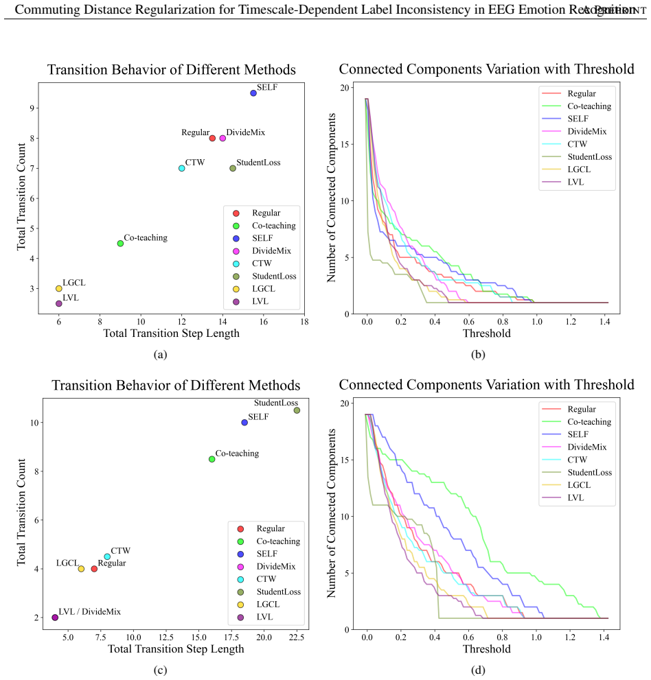
The machinery is an undirected emotion-level graph whose vertices are valence or arousal ratings and whose edges encode admissible transitions; the graph Laplacian L = D − A and its pseudoinverse L† appear as the kernel that turns prediction differences into squared commute-time distances. The two loss forms are LVL = (1/N) Σ_i (Ŷ(t_i) − Ŷ(t_{i−1}))^T L†(Ŷ(t_i) − Ŷ(t_{i−1})) and LGCL = (1/N) Σ_i (Ŷ(t_i) − E[Ŷ(t)])^T L†(Ŷ(t_i) − E[Ŷ(t)]). The commute-time distance theorem c_ij = vol(V)(e_i − e_j)^T L†(e_i − e_j) supplies the link to random walks, while the Transition Difficulty Postulate, the Intermediate Value Assumption, and the Full Expectation Assumption justify the line graph and the loss forms. The graph ablation shows that removing the graph degrades qualitative metrics, so the graph kernel carries the regularization effect.
What would settle it
Obtain EEG data with dense moment-by-moment emotion annotations aligned to the signal, train with and without LVL and LGCL, and compare per-segment predictions against those local ground-truth labels. The central claim is wrong if the regularized models do not show better agreement with the local labels, or if replacing the injected i.i.d. symmetric flips with autocorrelated label noise erases the ranking advantage.
Extended reading notes
Core claim
The central claim is that the timescale mismatch between short EEG segments and the global trial label—called Timescale-Dependent Label Inconsistency (TsDLI)—can be mitigated by penalizing the commute distance between consecutive local predictions (LVL) and between each local prediction and the trial-level expectation (LGCL), with the commute distance encoded by the pseudoinverse L† of an emotion-transition graph Laplacian. The paper further shows that these two losses are equivalent up to constants, so they act as one regularizer family rather than two independent mechanisms. In subject-dependent experiments with injected 20% and 40% symmetric label noise, LVL and LGCL rank first and second among eight training methods in a weighted Borda Count aggregation across three backbones, two datasets, and five metrics, while preserving or slightly improving F1 and Top-2 accuracy. The regularizers reduce implausible prediction jumps and are presented as a principled trade-off between quantitative accuracy and temporal plausibility.
Load-bearing premise
The benchmark simulates timescale-dependent label inconsistency by randomly flipping a portion of trial labels; if real label inconsistency is temporally correlated rather than random, the measured gains may not carry over to actual EEG recordings.
Editorial extensions
If this is right
- Adding LVL or LGCL to training changes the aggregate ranking: LVL ranks first and LGCL ranks second among eight methods across three backbones, two datasets, and two noise levels under the paper's weighted Borda Count aggregation.
- The regularizers improve qualitative consistency metrics (Ac, δd, vd) without sacrificing—and sometimes improving—F1 and Top-2 accuracy.
- Because the losses need no segment-level labels, they let existing trial-labeled EEG corpora be reused for consistency-regularized training.
- The two losses are equivalent up to constants, and the ablation with αLVL + βLGCL weights shows no statistically significant difference, so a practitioner need not tune both.
- Even a hand-crafted line graph prior suppresses implausible prediction jumps; dropping the graph worsens qualitative metrics.
Reading between the lines
- A testable extension beyond the paper: compare LVL and LGCL on a dataset with dense, time-aligned continuous emotion ratings; if the regularizers' advantage shrinks or reverses when evaluated against true moment-by-moment labels, the i.i.d. injection of symmetric flips was the reason for the gains.
- The same commute-distance kernel could regularize other weakly labeled temporal classification problems—action segmentation, speech-emotion recognition, or physiological monitoring—where coarse clip labels are inherited by short windows.
- The equivalence proof suggests LVL and LGCL are two views of one mechanism; learning the graph, and hence L†, per subject could turn the fixed line graph into an adaptive prior, which the paper lists as future work.
- Real TsDLI likely has autocorrelated structure; injecting temporally correlated noise rather than i.i.d. flips would test whether the method's advantage is an artifact of the noise model.
Editorial analysis
A structured set of objections, weighed in public.
Referee Report
Summary. The paper introduces Timescale-Dependent Label Inconsistency (TsDLI) in EEG emotion recognition, proposes two regularization losses, Local Variation Loss (LVL) and Local-Global Consistency Loss (LGCL), built on graph commute-time distances and a line-graph emotion transition prior, and defines new qualitative metrics (Ac, δd, vd) for evaluating temporal consistency. Experiments on DREAMER and DEAP with EEGNet, LSTM, and transformer backbones under 20% and 40% synthetic label noise compare six baselines plus LVL and LGCL, reporting that LVL achieves the best aggregate Borda rank and LGCL frequently ranks second. Appendix A provides an equivalence proof between LVL and LGCL.
Significance. If the empirical claims hold, the paper would contribute a principled, graph-theoretic regularizer for a realistic problem in EEG affect recognition, and its distinction between quantitative accuracy and qualitative temporal consistency is a useful framing. The commute-distance construction is mathematically self-contained, and the proposed losses are broadly applicable beyond EEG. However, the current evidence is weakened by the i.i.d. noise proxy, the partial circularity between the qualitative metrics and the proposed losses, the absence of a specified regularization weight, and the lack of significance testing.
major comments (4)
- [Section 4, Data Preprocessing] The experiments simulate TsDLI by randomly flipping a portion of inherited trial-level labels to alternative labels with equal probability (i.i.d. symmetric noise). This does not reproduce the temporally correlated, timescale-dependent discrepancy described in Section 1 and Figure 1, so the reported gains do not directly validate the central claim that LVL/LGCL mitigate TsDLI. Please add an experiment with temporally correlated label noise (e.g., block-structured flips or noise whose rate varies with segment position) or with any available segment-level annotations, and report results separately for the two noise regimes.
- [Sections 3.5 and 4, Evaluation Metrics and Borda Count] The qualitative metrics Ac, δd, and vd reward small adjacent prediction differences on hard labels, which is precisely the quantity that the LVL regularizer in Eq. (1) penalizes. Because these three metrics carry total weight 0.5 in the Borda aggregate and F1/Top2 carry 0.5, a model that outputs a near-constant prediction can achieve near-optimal qualitative scores by construction, even if it does not track the true local emotion state. Since test labels are inherited trial-level labels, no local ground truth is available to rule this out; the paper's limitation (4) concedes this. Please add a control experiment with a generic temporal-smoothing regularizer (e.g., total variation on softmax outputs with the Euclidean kernel), and report F1/Top2 and qualitative metrics both separately and jointly.
- [Sections 3.3-3.4 and 4] The total training objective is never specified: no value or search range is given for the regularization weight λ multiplying LVL or LGCL, and Table 2 only varies the relative weight α/β with the total weight implicit. Without this information the method is not reproducible, and the observed gains could be driven by the choice of λ rather than by the proposed regularizer. Please state the full loss, the λ/α/β values used in the main experiments, and a sensitivity analysis over λ.
- [Section 4, Main Results and Appendix B] All conclusions are based on averaged ranks or scores over 10 runs and 23/32 subjects, but no statistical significance tests are reported. Given the small per-subject test sets and the hand-weighted Borda aggregation, paired comparisons (e.g., Wilcoxon signed-rank tests across subjects or runs) with effect sizes or confidence intervals are needed to support claims such as 'LVL achieves the best aggregate rank across all benchmarked backbones and metrics'.
minor comments (5)
- [Section 4, Baselines] The text says 'five baseline methods' but then lists six: Regular, Co-teaching, SELF, DivideMix, CTW, and StudentLoss.
- [Appendix A, Eq. (33)] The constant in the second equivalence inequality appears mistyped: from the preceding line, the bound should be (N-1)^2 L1 rather than (N-1)^2/N L1 if L1 is defined by Eq. (11).
- [Section 3.4] The claim that L† is introduced 'in place of the standard identity matrix' is a modeling assumption rather than a consequence of the Full Expectation Assumption; the paper should state explicitly that this is a design choice, not a derivation.
- [Section 4.1, DEAP relabeling] The quartile-based relabeling of the 10-point DEAP scale into four bins changes the label space; please state explicitly that all reported DEAP numbers refer to the relabeled four-bin labels, and justify why this preprocessing does not itself remove the timescale-dependence being studied.
- [Appendix B] Figures 7-10 present the detailed rank tables as raster images; providing machine-readable numerical tables in the appendix would improve verifiability.
Circularity Check
The loss derivation is self-contained, but the validation loop is partially circular because the qualitative metrics are direct functions of the very adjacent-prediction differences that LVL minimizes, and these metrics carry half of the aggregate Borda weight.
-
self definitional
[Section 3.3, Eq. (1); Section 3.5 (definitions of vd, δd, Ac); Section 4, Evaluation Metrics (Borda weights)]
"Local Variation Loss (LVL): L= 1/N Σ_{i=1}^N (Ŷ(t_i)−Ŷ(t_{i−1}))^T L†(Ŷ(t_i)−Ŷ(t_{i−1})) ... vd := 1/N Σ_{i=1}^N |y_{i+1}−y_i| ... δd = max_{1≤i<n} |y_{i+1}−y_i| ... the two quantitative metrics (F1 score, Top-2 accuracy) are assigned a weight of 0.25 each, while three qualitative metrics (Ac, vd, δd) are weighted by 1/6, ensuring equal total weights (0.5) for both the quantitative and qualitative evaluations."
By construction, LVL penalizes the resistance-weighted difference between consecutive predictions, while the qualitative metrics vd, δd, and Ac are all monotonically decreasing functions of the same consecutive-prediction differences (in hard-label form). These three metrics receive half of the total Borda weight, so a model that learns to output nearly constant predictions both minimizes the LVL objective and automatically scores well on half of the aggregate ranking metric.
full rationale
The mathematical derivation of the proposed losses is not circular: LVL and LGCL are derived from stated assumptions (TDP, IVA, FEA) plus the classical commute-time distance identity, and the equivalence proof in Appendix A is a self-contained inequality argument. No load-bearing self-citations or imported uniqueness claims appear; the cited external works (e.g., Klein and Randić, Lovász) are standard results used as tools. The central circularity-adjacent issue is the evaluation loop. The paper introduces the qualitative metrics Ac, δd, and vd specifically to assess TsDLI, but these metrics are direct operationalizations of the same adjacent-prediction fluctuation magnitude that LVL is designed to suppress. Giving these three metrics half of the Borda weight means the aggregate ranking is largely predetermined toward the proposed regularizer, independent of whether the smoothed predictions correspond to true local emotions. The quantitative metrics (F1, Top-2) and the comparison against external baselines provide some independent content, which keeps the score moderate rather than severe. The paper's own limitation statements—that the regularizers do not infer time-resolved labels and that sparse ground truth prevents direct validation—further confirm that the qualitative metrics cannot be checked against an independent target. Overall, the derivation chain is sound, but the empirical confirmation of the central claim is partially definitional, yielding a partial circularity score of 4.
Assumptions & free parameters
free parameters (6)
- Emotion transition graph G0 (line graph with unit edge weights) =
1-2-3-4-5 path graph, all weights 1
- Graph edge-weight configurations G1, G2, GA =
G1: edges 1-2 and 4-5 carry half weight; G2: edges 2-3 and 3-4 carry half weight; GA: complete graph
- Regularization loss weight (lambda) =
Not stated
- Borda count metric weights =
F1 0.25, Top2 0.25, Ac 1/6, vd 1/6, delta_d 1/6
- Synthetic noise levels =
20% and 40% symmetric flips
- DEAP quartile relabeling into 4 bins =
Labels 0-9 mapped to quartiles 0-3
assumptions (7)
- domain assumption Transition Difficulty Postulate (TDP): transitions between emotional levels become less likely as numerical distance grows (Assumption 3.1).
- domain assumption Intermediate Value Assumption (IVA): any transition from i to j passes through intermediate levels (Assumption 3.2).
- domain assumption Full Expectation Assumption (FEA): Y_G = E_t[Y(t)] (Assumption 3.3).
- domain assumption Uniform density p(t) over segments when deriving LGCL (Section 3.4).
- ad hoc to paper The L† kernel can replace the identity matrix in the variance loss without changing the objective's interpretation (Section 3.4).
- standard math Graph Laplacian pseudoinverse is positive semi-definite and defines a valid commute-time/resistance distance (Klein-Randic theorem).
- standard math One-hot encoded labels combined with softmax cross-entropy; model outputs are prediction probabilities (Section 3).
Cite this review
Pith. "Pith review of Commuting Distance Regularization for Timescale-Dependent Label Inconsistency in EEG Emotion Recognition." pith.science (2026). https://pith.science/paper/EOYNSRHC
@misc{pith2026250710895,
  author       = {Pith},
  title        = {Pith review of: Commuting Distance Regularization for Timescale-Dependent Label Inconsistency in EEG Emotion Recognition},
  year         = {2026},
  howpublished = {\url{https://pith.science/paper/EOYNSRHC}},
  note         = {Machine review of arXiv:2507.10895}
}
read the original abstract
In this work, we address the often-overlooked issue of Timescale Dependent Label Inconsistency (TsDLI) in training neural network models for EEG-based human emotion recognition. To mitigate TsDLI and enhance model generalization and explainability, we propose two novel regularization strategies: Local Variation Loss (LVL) and Local-Global Consistency Loss (LGCL). Both methods incorporate classical mathematical principles--specifically, functions of bounded variation and commute-time distances--within a graph theoretic framework. Complementing our regularizers, we introduce a suite of new evaluation metrics that better capture the alignment between temporally local predictions and their associated global emotion labels. We validate our approach through comprehensive experiments on two widely used EEG emotion datasets, DREAMER and DEAP, across a range of neural architectures including LSTM and transformer-based models. Performance is assessed using five distinct metrics encompassing both quantitative accuracy and qualitative consistency. Results consistently show that our proposed methods outperform state-of-the-art baselines, delivering superior aggregate performance and offering a principled trade-off between interpretability and predictive power under label inconsistency. Notably, LVL achieves the best aggregate rank across all benchmarked backbones and metrics, while LGCL frequently ranks the second, highlighting the effectiveness of our framework.
Figures


Figures from the paper (7 more)




Reference graph
Works this paper leans on
-
[1]
M. Alvo and L. Philip. Statistical methods for ranking data, volume 1341. Springer, 2014
work page 2014
-
[2]
Berthelot, N
D. Berthelot, N. Carlini, I. Goodfellow, N. Papernot, A. Oliver, and C. A. Raffel. Mixmatch: A holistic approach to semi-supervised learning. Advances in neural information processing systems, 32, 2019
2019
-
[3]
T. Buda, A. Maki, and M. A. Mazurowski. A systematic study of the class imbalance problem in convolutional neural networks. Neural Networks, 106: 0 249--259, 2018
work page 2018
-
[4]
P.-C. B \"u rkner. On the information obtainable from comparative judgments. psychometrika, 87 0 (4): 0 1439--1472, 2022
work page 2022
-
[5]
E. D. Cubuk, B. Zoph, D. Mane, V. Vasudevan, and Q. V. Le. Autoaugment: Learning augmentation strategies from data. In Proceedings of the IEEE Conference on Computer Vision and Pattern Recognition (CVPR), pages 113--123, 2019
work page 2019
-
[6]
H. Cui, A. Liu, X. Zhang, X. Chen, K. Wang, and X. Chen. Eeg-based emotion recognition using an end-to-end regional-asymmetric convolutional neural network. Knowledge-Based Systems, 205: 0 106243, 2020
work page 2020
-
[7]
R. J. Davidson. Affective style and affective disorders: Perspectives from affective neuroscience. Cognition & emotion, 12 0 (3): 0 307--330, 1998
work page 1998
-
[8]
I. Douven. A bayesian perspective on likert scales and central tendency. Psychonomic bulletin & review, 25: 0 1203--1211, 2018
work page 2018
Show all 53 references
-
[9]
Drot \'a r, M
P. Drot \'a r, M. Gazda, and J. Gazda. Heterogeneous ensemble feature selection based on weighted B orda c ount. In 2017 9th International Conference on Information Technology and Electrical Engineering (ICITEE), pages 1--4. IEEE, 2017
2017
-
[10]
Duan, J.-Y
R.-N. Duan, J.-Y. Zhu, and B.-L. Lu. Differential entropy feature for EEG -based emotion classification. In 6th International IEEE/EMBS Conference on Neural Engineering (NER), pages 81--84. IEEE, 2013
2013
-
[11]
Furlanello, Z
T. Furlanello, Z. C. Lipton, M. Tschannen, L. Itti, and A. Anandkumar. Born again neural networks. In International Conference on Machine Learning (ICML), pages 1607--1616, 2018
2018
-
[12]
Ghosh, H
A. Ghosh, H. Kumar, and P. S. Sastry. Robust loss functions under label noise for deep neural networks. In Proceedings of the AAAI conference on artificial intelligence, volume 31, 2017
2017
-
[13]
Goodfellow, Y
I. Goodfellow, Y. Bengio, A. Courville, and Y. Bengio. Deep learning, volume 1. MIT press Cambridge, 2016
2016
-
[14]
Gutentag, O
T. Gutentag, O. P. John, J. J. Gross, and M. Tamir. Incremental theories of emotion across time: Temporal dynamics and correlates of change. Emotion, 22 0 (6): 0 1137, 2022
2022
-
[15]
B. Han, Q. Yao, X. Yu, G. Niu, M. Xu, W. Hu, I. Tsang, and M. Sugiyama. Co-teaching: Robust training of deep neural networks with extremely noisy labels. Advances in neural information processing systems, 31, 2018
2018
-
[16]
Janocha and W
K. Janocha and W. M. Czarnecki. On loss functions for deep neural networks in classification. arXiv preprint arXiv:1702.05659, 2017
2017 arXiv
-
[17]
Katsigiannis and N
S. Katsigiannis and N. Ramzan. Dreamer: A database for emotion recognition through eeg and ecg signals from wireless low-cost off-the-shelf devices. IEEE journal of biomedical and health informatics, 22 0 (1): 0 98--107, 2017
2017
-
[18]
D. J. Klein and M. Randić. Resistance distance. Journal of Mathematical Chemistry, 12: 0 81--95, 1993
1993
-
[19]
Koelstra, C
S. Koelstra, C. Muhl, M. Soleymani, J.-S. Lee, A. Yazdani, T. Ebrahimi, T. Pun, A. Nijholt, and I. Patras. Deap: A database for emotion analysis; using physiological signals. IEEE transactions on affective computing, 3 0 (1): 0 18--31, 2011
2011
-
[20]
Kuppens and P
P. Kuppens and P. Verduyn. Emotion dynamics. Current Opinion in Psychology, 17: 0 22--26, 2017
2017
-
[21]
V. J. Lawhern, A. J. Solon, N. R. Waytowich, S. M. Gordon, C. P. Hung, and B. J. Lance. Eegnet: a compact convolutional neural network for eeg-based brain--computer interfaces. Journal of neural engineering, 15 0 (5): 0 056013, 2018
2018
-
[22]
F. Li, H. Xu, C. Wu, et al. Learning from noisy labels with distillation. In International Joint Conference on Artificial Intelligence (IJCAI), 2021
2021
-
[23]
J. Li, R. Socher, and S. C. Hoi. Dividemix: Learning with noisy labels as semi-supervised learning. arXiv preprint arXiv:2002.07394, 2020
2002 arXiv
-
[24]
X. Li, Y. Zhang, P. Tiwari, D. Song, B. Hu, M. Yang, Z. Zhao, N. Kumar, and P. Marttinen. EEG based emotion recognition: A tutorial and review. ACM Computing Surveys, 55 0 (4): 0 1--57, 2022
2022
-
[25]
C. Liu, X. Zhou, Z. Zhu, L. Zhai, Z. Jia, and Y. Liu. Vbh-gnn: variational bayesian heterogeneous graph neural networks for cross-subject emotion recognition. In The Twelfth International Conference on Learning Representations, 2024
2024
-
[26]
Z. Liu, D. Chen, W. Pei, Q. Ma, et al. Scale-teaching: Robust multi-scale training for time series classification with noisy labels. Advances in Neural Information Processing Systems, 36: 0 33726--33757, 2023
2023
-
[27]
Lov \'a sz
L. Lov \'a sz. Random walks on graphs. Combinatorics, Paul erdos is eighty, 2 0 (1-46): 0 4, 1993
1993
-
[28]
P. Ma, Z. Liu, J. Zheng, L. Wang, and Q. Ma. CTW : C onfident T ime- W arping for T ime- S eries L abel- N oise L earning. In IJCAI, pages 4046--4054, 2023
2023
-
[29]
D. T. Nguyen, C. K. Mummadi, T. P. N. Ngo, T. H. P. Nguyen, L. Beggel, and T. Brox. Self: Learning to filter noisy labels with self-ensembling. arXiv preprint arXiv:1910.01842, 2019
1910 arXiv
-
[30]
Pallasdies, P
F. Pallasdies, P. Norton, J.-H. Schleimer, and S. Schreiber. Neural optimization: Understanding trade-offs with pareto theory. Current opinion in neurobiology, 71: 0 84--91, 2021
2021
-
[31]
Patrini, A
G. Patrini, A. Rozza, A. K. Menon, R. Nock, and L. Qu. Making deep neural networks robust to label noise: A loss correction approach. In Proceedings of the IEEE Conference on Computer Vision and Pattern Recognition (CVPR), pages 1944--1952, 2017
1944
-
[32]
D. L. Paulhus, S. Vazire, et al. The self-report method. Handbook of research methods in personality psychology, 1 0 (2007): 0 224--239, 2007
2007
-
[33]
N. A. Puccetti, W. J. Villano, J. P. Fadok, and A. S. Heller. Temporal dynamics of affect in the brain: Evidence from human imaging and animal models. Neuroscience & Biobehavioral Reviews, 133: 0 104491, 2022
2022
-
[34]
M. Ren, W. Zeng, B. Yang, and R. Urtasun. Learning to reweight examples for robust deep learning. In International Conference on Machine Learning (ICML), pages 4334--4343, 2018
2018
-
[35]
D. G. Saari. The optimal ranking method is the B orda C ount. Technical report, Discussion paper, 1985
1985
-
[36]
W. E. Saris and I. N. Gallhofer. Design, evaluation, and analysis of questionnaires for survey research. John Wiley & Sons, 2014
2014
-
[37]
K. R. Scherer. The dynamic architecture of emotion: Evidence for the component process model. Cognition and emotion, 23 0 (7): 0 1307--1351, 2009
2009
-
[38]
H. Song, J. Choi, and I. Y. Lee. Multi-class learning from noisy partial labels. IEEE Transactions on Neural Networks and Learning Systems, 32 0 (12): 0 5600--5613, 2021
2021
-
[39]
H. Song, M. Kim, D. Park, Y. Shin, and J.-G. Lee. Learning from noisy labels with deep neural networks: A survey. IEEE transactions on neural networks and learning systems, 34 0 (11): 0 8135--8153, 2022
2022
-
[40]
R. Song, Y. Li, Y. Jia, Y. Wang, and P. Rao. Efficient, robust and divisible paired comparison for subjective quality assessment. Multimedia Tools and Applications, 77: 0 13597--13613, 2018
2018
-
[41]
Tanaka, D
D. Tanaka, D. Ikami, T. Yamasaki, and K. Aizawa. Joint optimization framework for learning with noisy labels. In Proceedings of the IEEE Conference on Computer Vision and Pattern Recognition (CVPR), pages 5552--5560, 2018
2018
-
[42]
Tarvainen and H
A. Tarvainen and H. Valpola. Mean teachers are better role models: Weight-averaged consistency targets improve semi-supervised deep learning results. In Advances in Neural Information Processing Systems (NeurIPS), pages 1195--1204, 2017
2017
-
[43]
Tourangeau, L
R. Tourangeau, L. J. Rips, and K. Rasinski. The psychology of survey response. Cambridge University Press, 2000
2000
-
[44]
Von Luxburg
U. Von Luxburg. A tutorial on spectral clustering. Statistics and computing, 17: 0 395--416, 2007
2007
-
[45]
Q. Wang, Y. Ma, K. Zhao, and Y. Tian. A comprehensive survey of loss functions in machine learning. Annals of Data Science, pages 1--26, 2020
2020
-
[46]
Y. Wang, X. Ma, Z. Chen, Y. Luo, J. Yi, and J. Bailey. Symmetric cross entropy for robust learning with noisy labels. In Proceedings of the IEEE/CVF international conference on computer vision, pages 322--330, 2019
2019
-
[47]
Z. Wang, D. Sun, S. Zhou, H. Wang, J. Fan, L. Huang, and J. Bu. Noisy GL : A C omprehensive B enchmark for G raph N eural N etworks under L abel N oise. Advances in Neural Information Processing Systems, 37: 0 38142--38170, 2025
2025
-
[48]
C. E. Waugh, E. Z. Shing, and B. M. Avery. Temporal dynamics of emotional processing in the brain. Emotion Review, 7 0 (4): 0 323--329, 2015
2015
-
[49]
Xie, M.-T
Q. Xie, M.-T. Luong, E. Hovy, and Q. V. Le. Self-training with noisy student improves imagenet classification. In Proceedings of the IEEE/CVF Conference on Computer Vision and Pattern Recognition (CVPR), pages 10687--10698, 2020
2020
-
[50]
T. Yue, S. Xue, X. Gao, Y. Tang, L. Guo, J. Jiang, and J. Liu. Eegpt: Unleashing the potential of eeg generalist foundation model by autoregressive pre-training. arXiv preprint arXiv:2410.19779, 2024
2024 arXiv
-
[51]
Zhang, J.-Q
S. Zhang, J.-Q. Li, H. Fujita, Y.-W. Li, D.-B. Wang, T.-T. Zhu, M.-L. Zhang, and C.-Y. Liu. Student loss: Towards the probability assumption in inaccurate supervision. IEEE Transactions on Pattern Analysis and Machine Intelligence, 46 0 (6): 0 4460--4475, 2024
2024
-
[52]
Zhang and M
Z. Zhang and M. Sabuncu. Generalized cross entropy loss for training deep neural networks with noisy labels. Advances in neural information processing systems, 31, 2018
2018
-
[53]
Zheng and B.-L
W.-L. Zheng and B.-L. Lu. Investigating critical frequency bands and channels for eeg-based emotion recognition with deep neural networks. IEEE Transactions on autonomous mental development, 7 0 (3): 0 162--175, 2015
2015
Reviewed August 6, 2026 · model on record in the stance chip above.
Discussion (0). Sign in to comment.