REVIEW 2 major objections 5 minor 50 references
Solar disk gamma-rays emission via synthetic magnetic field from photosphere to low corona
T0 review · 2 major / 5 minor · reviewed 2026-08-06 · deepseek-v4-flash
Pith's one-line read Braided magnetic fields explain the Sun's gamma-ray spectrum above 10 GeV
desk verdict New synthetic braided-field model reproduces the solar-disk gamma-ray spectrum, but the key rebrightening is likely driven by an isotropic injection at the photosphere that bypasses the physical mirroring filter. read the letter →
The pith
A machine-rendered reading of the paper's core claim, the machinery that carries it, and where it could break.
The reading
What carries the argument
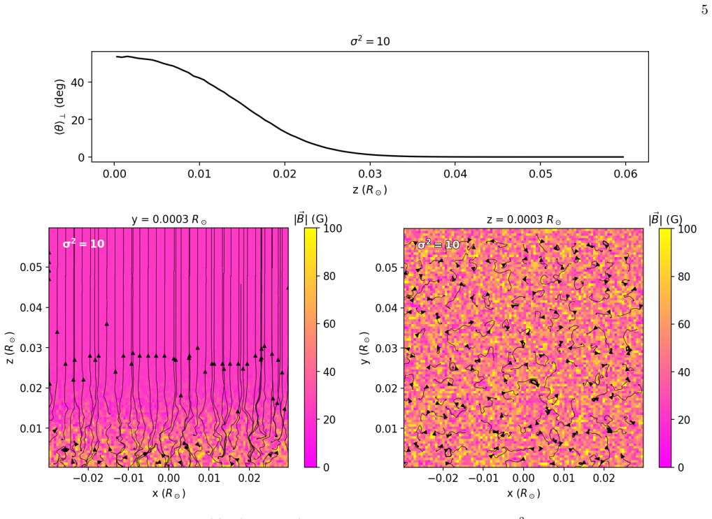
The load-bearing object is the synthetic total magnetic field $\mathbf{B}(x,y,z) = B_0\hat{k} + \nabla\times[f(z)\mathbf{S}(x,y,z)]$, a divergence-free superposition of a uniform vertical field and a plane-wave vector potential $\mathbf{S}$ whose amplitude is modulated by the Gaussian envelope $f(z)=e^{-(z/\Lambda)^2}$. This envelope confines the braiding to a layer of height $\Lambda\simeq 1.41\times10^{-2}R_\odot$ above the photosphere, so the field is laminar in the corona and progressively horizontal and tangled near the surface. The braiding amplitude $\sigma^2=\langle\delta B^2\rangle/B_0^2$, with values 0.1, 1, and 10, controls the fraction of cosmic rays that interact before escaping, which is the quantity that directly sets the gamma-ray flux and its spectral shape.
What would settle it
Recompute the same test-particle gamma-ray transport using a braided magnetic field extracted from a time-dependent, high-resolution MHD simulation of the photosphere and chromosphere, and check whether the 30-100 GeV flattening survives; if it does not, the synthetic geometry is responsible for the rebrightening rather than real solar physics. Alternatively, a future Fermi-LAT/HAWC measurement with better statistics that shows a deepening dip and no rebrightening in the 30-100 GeV range would directly contradict the prediction.
Extended reading notes
Core claim
The central claim is that open, increasingly braided field lines alone, without closed magnetic arcades, can account for the >10 GeV solar-disk gamma-ray spectrum, and that the rebrightening between approximately 30 and 100 GeV is a physical consequence of enhanced cosmic-ray confinement in the photo- and chromosphere. The magnetic field is built as $\mathbf{B} = B_0\hat{k} + \nabla\times[f(z)\mathbf{S}(x,y,z)]$ with $f(z)=e^{-(z/\Lambda)^2}$ and $\Lambda \simeq 1.41\times 10^{-2}R_\odot$, so distortions grow only near the surface; the braiding strength $\sigma^2 = \langle\delta B^2\rangle/B_0^2$ controls how horizontal the field becomes. In the simulations, the fraction of injected protons that interact rises with $\sigma^2$ when particles start inside the braided layer, raising the gamma-ray yield and flattening the dip, and this flattening saturates at $\sigma^2\gtrsim 10$ rather than growing into a bump. The authors take the saturation, together with tests changing $L_s$ and $\Lambda$, as evidence that the dip-rebrightening is a genuine physical effect tied to the condition $r_g(300\,\mathrm{GeV}) \simeq L_s$.
Load-bearing premise
The load-bearing assumption is that the synthetic static field, with its Gaussian vertical envelope and plane-wave distortions, is a faithful stand-in for the real photospheric and chromospheric field; if the actual field has time-dependent or smaller-scale structure not captured by this construction, the calculated trapping and the predicted rebrightening could fail.
Editorial extensions
If this is right
- The >10 GeV solar-disk gamma-ray spectrum is set by magnetic geometry, not by the cosmic-ray injection spectrum, so spectral features like the ~30 GeV dip become diagnostics of photospheric field structure.
- Stronger braiding raises the gamma-ray flux at all energies and specifically flattens the 30-100 GeV dip, so the dip depth should vary with solar-cycle phase and with local magnetic complexity in time-resolved observations.
- Open braided field lines alone can account for the observed flux, meaning closed magnetic arcades are not required to explain the >10 GeV emission.
- The model predicts an energy-dependent angular pattern: higher-energy gamma-rays are emitted nearly tangent to the solar surface while lower-energy emission is more isotropic, consistent with the Fermi-LAT morphology.
- The relation $r_g(300\,\mathrm{GeV}) \simeq L_s$ ties the dip energy to the granular scale of photospheric magnetic structures, making the dip a measurable scale of the low solar atmosphere.
Reading between the lines
- If braiding strength is the controlling parameter, the depth of the 30-100 GeV dip should vary across the solar cycle and with heliographic latitude, a testable prediction beyond the paper's static snapshot.
- The same trapped galactic-cosmic-ray population would also produce solar-disk neutrons and neutrinos at similar energies, so the braiding model could be cross-checked with non-gamma-ray channels.
- Because the grid resolution (~418 km) excludes structures below the granular scale, the sub-10 GeV flux and possibly the dip shape could change once smaller-scale field variations are resolved; the central claim is safest above 10 GeV.
- Replacing the synthetic field with a braided field taken from an MHD simulation of convective flows would show whether the Gaussian envelope is essential or whether any braided open-field geometry yields the same rebrightening.
Editorial analysis
A structured set of objections, weighed in public.
Referee Report
Summary. This manuscript presents 3D test-particle simulations of galactic cosmic-ray protons in a synthetic, divergence-free magnetic field that is open at the top and increasingly braided toward the photosphere. Protons are injected isotropically at two heights, one in the laminar corona and one in the braided photosphere; the fraction that undergoes p-p interactions is used to rescale the observed local interstellar GCR spectrum and to compute the solar disk gamma-ray flux via Eq. (10). The main finding is that with increasing braiding amplitude, the interaction fraction for particles injected in the braided layer grows, leading to a flattening/rebrightening of the flux in the 30-100 GeV range, which the authors interpret as a physical confinement effect and compare with Fermi-LAT and HAWC data.
Significance. If the central claim were established, the paper would offer a plausible explanation for the spectral dip/rebrightening in the 30-100 GeV range of the solar disk gamma-ray emission using an open-field braided geometry, complementing the closed-arcade model of Puzzoni et al. (2024). The computational setup is transparent, the synthetic field construction is explicitly separated from the particle transport, and the model parameters are anchored to solar magnetometry rather than fitted to gamma-ray data. The sensitivity study over sigma^2, Ls, and Lambda is a useful diagnostic. However, the physical interpretation is critically dependent on the particle injection scheme, which as argued above may introduce an artificial source of interacting particles; until this is resolved, the significance of the claimed rebrightening mechanism remains uncertain.
major comments (2)
- [3.2, Eq. (10), and Fig. 3] The averaging of Nint/Ninj over injections at z_up and z_down is not physically justified. In the real solar atmosphere, the phase-space density of GCRs at the photosphere is the filtered remnant of the external isotropic population that has propagated downward through the mirroring and escape regions; it is not an independent isotropic source. The injection at z_down therefore loads the braided layer with particles that would not be present in the steady-state distribution, artificially enhancing the interaction probability. This is not a cosmetic issue: Fig. 3 shows that Nint increases with sigma^2 only for the z_down injection, while the z_up injection is nearly independent of sigma^2, and Eq. (10) uses their average. Consequently, the claimed 30-100 GeV rebrightening in Sec. 4.3 is driven by an artificial source term. The authors should either (i) inject particles only at the top boundary and count those that subsequently interact, or (ii) weight the z_down contribution by the transmission probability computed from the z_up transport; the resulting spectral shape should be compared to show that the rebrightening is not a boundary artifact.
- [4.3 and Fig. 5] Because Eq. (10) uses the full observed local interstellar GCR intensity for both injection altitudes, the absolute gamma-ray flux in Fig. 5 is normalized by a particle population at z_down that is not supplied from infinity. The factor 2πR_sun^2/L^2 in the flux expression assumes the injection surface area equals the domain cross-section, but the z_down injection does not correspond to an incident flux at that height. The apparent agreement with the Fermi-LAT/HAWC points in Fig. 5 is therefore not a model prediction that is independent of the injection scheme. The requested top-boundary test is also needed to establish whether the absolute flux level remains compatible with the observations.
minor comments (5)
- [Abstract] The abstract uses 'Fermi-HAWC' while the standard notation in the text is 'Fermi-LAT/HAWC'; please make it consistent.
- [Section 3.2] The justification of isotropic injection by the observed isotropy of anomalous cosmic rays at ~0.1 AU (Rankin 2024) is not directly applicable to GeV-TeV galactic cosmic rays at the photosphere, where the Sun's absorbing boundary creates a loss cone; please clarify or replace this justification.
- [Section 4.3] The discussion of the Ls scan states that increasing Ls to 3 Ls 'does not change the flux at the dip' after arguing that the dip-rebrightening is associated with rg(300 GeV) ~ Ls; this tension should be resolved by stating explicitly which mechanism (resonance vs mean free path) controls the effect.
- [Section 2.1] The phrase 'the ratio between this Alfvén velocity to the particle speed' should read 'the ratio of this Alfvén velocity to the particle speed'.
- [Figure 5] The color coding of the different sigma^2 curves should be described in the caption; the text refers to green, brown, orange diamonds, and orange stars, but the caption as printed does not list them.
Circularity Check
No significant circularity: model parameters come from solar magnetometry; the gamma-ray comparison is an independent forward calculation against Fermi/HAWC data.
full rationale
The derivation chain is: construct a synthetic divergence-free field via Eqs. (1)-(8) with parameters B0, sigma^2, Ls, and Lambda chosen to emulate observed/MHD solar magnetic properties (e.g., horizontal-to-vertical field ratios, granular scales), not fitted to gamma-ray data; integrate test-particle proton orbits in that static field (Sec. 3); simulate Nint/Ninj as an output (Fig. 3, left); and fold it with the independently measured AMS/ISS-CREAM GCR spectrum and standard pp->pi0->gamma yields (Eq. 10) to compare against Fermi-LAT/HAWC flux (Fig. 5). No target quantity is defined in terms of itself: the simulated interaction fraction is not fitted to the observed gamma-ray spectrum, and the 30-100 GeV flattening tracks the simulated sigma^2 dependence of confinement, especially for z_down injection. The self-references (Puzzoni et al. 2024; Giacalone 2021; Giacalone & Jokipii 1999) supply the density profile, the flux-convolution method, and the Fourier-mode field superposition; these are methodological inputs, not a uniqueness theorem or a fitted prediction, and the central comparison remains against external Fermi-LAT/HAWC data. The paper explicitly acknowledges limitations (no closed field lines, no time dependence, unresolved sub-10 GeV structures, unspecified braiding driver), and these are modeling caveats rather than evidence of circular reasoning. The possible concern that z_down injection bypasses the coronal mirror filter is a boundary-condition/physics caveat, not a definitional reduction, so it does not raise the circularity score.
Assumptions & free parameters
free parameters (4)
- sigma^2 (relative magnetic fluctuation amplitude) =
scanned 0.1, 1, 10, 50; best match at 10
- B0 (background magnetic field strength) =
5 G and 50 G
- Ls (largest horizontal scale of magnetic structures) =
0.003 R_sun (about 2 Mm)
- Lambda (scale height of braiding onset) =
1.41e-2 R_sun
assumptions (4)
- ad hoc to paper The synthetic field B(x,y,z) in Eqs. (1)-(8) with f(z)=exp(-(z/Lambda)^2) approximates the real solar atmospheric field.
- domain assumption The magnetic field is static over the GCR propagation timescale (tens of seconds).
- domain assumption GCRs are injected isotropically at the two heights.
- standard math The density profile and the p-p interaction cross section and yield functions are accurate.
Cite this review
Pith. "Pith review of Solar disk gamma-rays emission via synthetic magnetic field from photosphere to low corona." pith.science (2026). https://pith.science/paper/QPPWF52F
@misc{pith2026250715468,
  author       = {Pith},
  title        = {Pith review of: Solar disk gamma-rays emission via synthetic magnetic field from photosphere to low corona},
  year         = {2026},
  howpublished = {\url{https://pith.science/paper/QPPWF52F}},
  note         = {Machine review of arXiv:2507.15468}
}
abstract
Gamma-ray emission in the GeV-TeV range from the solar disk is likely to arise from collisions of galactic cosmic rays (GCRs) with solar atmospheric plasma. In a previous study, we demonstrated that closed turbulent magnetic arcades trap efficiently GCRs leading to a gamma-ray flux consistent with the Fermi-HAWC observations (from $\sim 0.1$ GeV to $\sim 1$ TeV). Here, we model a synthetic magnetic field with a static, laminar structure of open field lines in the chromosphere increasingly braiding near the solar surface, with a scale height of $\sim 10^{-2} R_\odot$. The height-dependent increase in magnetic field line braiding is modulated by an exponential scalar function, mimicking the bending of the photo- and chromo-spheric magnetic field revealed by polarimetric observations and reproduced by MHD simulations. Employing 3D test-particle numerical simulations, we investigate how distorted magnetic field lines affect the gamma-rays production by injecting GeV-TeV protons into both magnetically laminar and braided regions. We find that with the chosen spatial resolution this synthetic magnetic field can account for the $> 10$ GeV gamma-ray spectrum observed by Fermi-LAT/HAWC. A rebrightening between approximately $30$ and $100$ GeV (following a $\sim 30$ GeV spectral dip), suggests an enhanced confinement within the photo-/chromospheric layer by a stronger braiding.
Figures


Figures from the paper (2 more)


Reference graph
Works this paper leans on
-
[1]
A., Ackermann, M., Ajello, M., et al
Abdo, A. A., Ackermann, M., Ajello, M., et al. 2011, ApJ, 736, 131, doi: 10.1088/0004-637X/736/2/131
-
[2]
U., Alfaro, R., Alvarez, C., et al
Abeysekara, A. U., Alfaro, R., Alvarez, C., et al. 2013, Astroparticle Physics, 50, 26, doi: 10.1016/j.astropartphys.2013.08.002
-
[3]
Puzzling Variation of Gamma Rays from the Sun over the Solar Cycle Revealed with Fermi-LAT
Acharyya, A., Adelfio, A., Ajello, M., et al. 2025, arXiv e-prints, arXiv:2505.06348, doi: 10.48550/arXiv.2505.06348
work page Pith review arXiv doi:10.48550/arxiv.2505.06348 2025
-
[4]
2021, PhR, 894, 1, doi: 10.1016/j.physrep.2020.09.003
Aguilar, M., Ali Cavasonza, L., Ambrosi, G., et al. 2021, PhR, 894, 1, doi: 10.1016/j.physrep.2020.09.003
-
[5]
2023, PhRvL, 131, 051201, doi: 10.1103/PhysRevLett.131.051201
Albert, A., Alfaro, R., Alvarez, C., et al. 2023, PhRvL, 131, 051201, doi: 10.1103/PhysRevLett.131.051201
-
[6]
Alfaro, R., Alvarez, C., Arteaga-Vel´ azquez, J. C., et al. 2024, ApJ, 966, 67, doi: 10.3847/1538-4357/ad3208
-
[7]
Amenomori, M., Bi, X. J., Chen, D., et al. 2018, PhRvL, 120, 031101, doi: 10.1103/PhysRevLett.120.031101
-
[8]
2023, A&A, 676, A112, doi: 10.1051/0004-6361/202346016
Antolin, P., Dolliou, A., Auch` ere, F., et al. 2023, A&A, 676, A112, doi: 10.1051/0004-6361/202346016
Show all 50 references
-
[9]
2024, ApJ, 962, 52, doi: 10.3847/1538-4357/ad1bd2
Arsioli, B., & Orlando, E. 2024, ApJ, 962, 52, doi: 10.3847/1538-4357/ad1bd2
2024 doi
-
[10]
Athay, R. G. 1976, The solar chromosphere and corona: Quiet sun, Vol. 53, doi: 10.1007/978-94-010-1715-2
1976 doi
-
[11]
B., Abdo, A
Atwood, W. B., Abdo, A. A., Ackermann, M., et al. 2009, ApJ, 697, 1071, doi: 10.1088/0004-637X/697/2/1071 Becker Tjus, J., Desiati, P., D¨ opper, N., et al. 2020, A&A, 633, A83, doi: 10.1051/0004-6361/201936306
2009 doi
-
[12]
K., & Langdon, A
Birdsall, C. K., & Langdon, A. B. 1991, Plasma Physics via Computer Simulation
1991
-
[13]
Cannady, N. W. 2022, in 37th International Cosmic Ray Conference, 604, doi: 10.22323/1.395.0604
2022 doi
-
[14]
H., Seo, E
Choi, G. H., Seo, E. S., Aggarwal, S., et al. 2022, ApJ, 940, 107, doi: 10.3847/1538-4357/ac9d2c
2022 doi
-
[15]
Danilovic, S., Sch¨ ussler, M., & Solanki, S. K. 2010, A&A, 513, A1, doi: 10.1051/0004-6361/200913379 del Pino Alem´ an, T., Trujillo Bueno, J.,ˇStˇ ep´ an, J., &
2010 doi
-
[16]
2018, ApJ, 863, 164, doi: 10.3847/1538-4357/aaceab D¨ orner, J., Morejon, L., Kampert, K.-H., & Becker Tjus, J
Shchukina, N. 2018, ApJ, 863, 164, doi: 10.3847/1538-4357/aaceab D¨ orner, J., Morejon, L., Kampert, K.-H., & Becker Tjus, J. 2025, JCAP, 2025, 043, doi: 10.1088/1475-7516/2025/04/043
2018 doi
-
[17]
2001, A&A, 378, 627, doi: 10.1051/0004-6361:20011263
Faurobert, M., Arnaud, J., Vigneau, J., & Frisch, H. 2001, A&A, 378, 627, doi: 10.1051/0004-6361:20011263
2001 doi
-
[18]
1995, A&A, 298, 289
Petrovay, K., & Spielfiedel, A. 1995, A&A, 298, 289
1995
-
[19]
M., Avrett, E
Fontenla, J. M., Avrett, E. H., & Loeser, R. 1993, ApJ, 406, 319, doi: 10.1086/172443
1993 doi
-
[20]
D., Drake, J
Fraschetti, F., Alvarado-G´ omez, J. D., Drake, J. J., Cohen, O., & Garraffo, C. 2022, ApJ, 937, 126, doi: 10.3847/1538-4357/ac86d7
2022 doi
-
[21]
Fraschetti, F., & Jokipii, J. R. 2011, ApJ, 734, 83, doi: 10.1088/0004-637X/734/2/83
2011 doi
-
[22]
2021, ApJ, 912, 83, doi: 10.3847/1538-4357/abf0b2
Giacalone, J. 2021, ApJ, 912, 83, doi: 10.3847/1538-4357/abf0b2
2021 doi
-
[23]
Giacalone, J., & Jokipii, J. R. 1999, ApJ, 520, 204, doi: 10.1086/307452 Gonz´ alez-Avil´ es, J. J., Guzm´ an, F. S., Fedun, V., et al. 2018, ApJ, 856, 176, doi: 10.3847/1538-4357/aab36f Gonz´ alez-Avil´ es, J. J., Murawski, K., Srivastava, A. K.,
1999 doi
-
[24]
V., & Gonz´ alez-Esparza, J
Zaqarashvili, T. V., & Gonz´ alez-Esparza, J. A. 2021, MNRAS, 505, 50, doi: 10.1093/mnras/stab1261 11 Guti´ errez, M., Masip, M., & Mu˜ noz, S. 2022, ApJ, 941, 86, doi: 10.3847/1538-4357/aca020
2021 doi
-
[25]
S., MacKinnon, A., Szydlarski, M., & Carlsson, M
Hudson, H. S., MacKinnon, A., Szydlarski, M., & Carlsson, M. 2020, MNRAS, 491, 4852, doi: 10.1093/mnras/stz3373
2020 doi
-
[26]
2021, Science Advances, 7, eabe8406, doi: 10.1126/sciadv.abe8406
Ishikawa, R., Trujillo Bueno, J., del Pino Alem´ an, T., et al. 2021, Science Advances, 7, eabe8406, doi: 10.1126/sciadv.abe8406
2021 doi
-
[27]
M., & Vila, G
Kafexhiu, E., Aharonian, F., Taylor, A. M., & Vila, G. S. 2014, PhRvD, 90, 123014, doi: 10.1103/PhysRevD.90.123014
2014 doi
-
[28]
R., Aharonian, F
Kelner, S. R., Aharonian, F. A., & Bugayov, V. V. 2006, PhRvD, 74, 034018, doi: 10.1103/PhysRevD.74.034018
2006 doi
-
[29]
F., Griffith, S., & Peter, A
Li, J.-T., Beacom, J. F., Griffith, S., & Peter, A. H. G. 2024a, ApJ, 961, 167, doi: 10.3847/1538-4357/ad158f
-
[30]
Li, Z., Ng, K. C. Y., Chen, S., Nan, Y., & He, H. 2024b, Chinese Physics C, 48, 045101, doi: 10.1088/1674-1137/ad1cda
-
[31]
F., Peter, A
Linden, T., Beacom, J. F., Peter, A. H. G., et al. 2022, PhRvD, 105, 063013, doi: 10.1103/PhysRevD.105.063013
2022 doi
-
[32]
F., et al
Linden, T., Zhou, B., Beacom, J. F., et al. 2018, PhRvL, 121, 131103, doi: 10.1103/PhysRevLett.121.131103
2018 doi
-
[33]
N., Luque, P
Mazziotta, M. N., Luque, P. D. L. T., Di Venere, L., et al. 2020, PhRvD, 101, 083011, doi: 10.1103/PhysRevD.101.083011
2020 doi
-
[34]
2007, ApJS, 170, 228, doi: 10.1086/513316
Mignone, A., Bodo, G., Massaglia, S., et al. 2007, ApJS, 170, 228, doi: 10.1086/513316
2007 doi
-
[35]
2018, ApJ, 859, 13, doi: 10.3847/1538-4357/aabccd
Mignone, A., Bodo, G., Vaidya, B., & Mattia, G. 2018, ApJ, 859, 13, doi: 10.3847/1538-4357/aabccd
2018 doi
-
[36]
2012, ApJS, 198, 7, doi: 10.1088/0067-0049/198/1/7
Mignone, A., Zanni, C., Tzeferacos, P., et al. 2012, ApJS, 198, 7, doi: 10.1088/0067-0049/198/1/7
2012 doi
-
[37]
J., Sharma, R., Tajfirouze, E., & Miriyala, H
Morton, R. J., Sharma, R., Tajfirouze, E., & Miriyala, H. 2023, Reviews of Modern Plasma Physics, 7, 17, doi: 10.1007/s41614-023-00118-3
2023 doi
-
[38]
Ng, K. C. Y., Beacom, J. F., Peter, A. H. G., & Rott, C. 2016, PhRvD, 94, 023004, doi: 10.1103/PhysRevD.94.023004
2016 doi
- [39]
-
[40]
2024, ApJ, 973, 118, doi: 10.3847/1538-4357/ad65ea
Puzzoni, E., Fraschetti, F., K´ ota, J., & Giacalone, J. 2024, ApJ, 973, 118, doi: 10.3847/1538-4357/ad65ea
2024 doi
-
[41]
Rankin, J. S. 2024, in AGU Fall Meeting Abstracts, Vol. 2024, SH21C–2832
2024
-
[42]
2014, Living Reviews in Solar Physics, 11, 4, doi: 10.12942/lrsp-2014-4
Reale, F. 2014, Living Reviews in Solar Physics, 11, 4, doi: 10.12942/lrsp-2014-4
2014 doi
-
[43]
2014, ApJ, 789, 132, doi: 10.1088/0004-637X/789/2/132
Rempel, M. 2014, ApJ, 789, 132, doi: 10.1088/0004-637X/789/2/132
2014 doi
-
[44]
A., Petrie, G., Kuhn, J., et al
Schad, T. A., Petrie, G., Kuhn, J., et al. 2024, Science Advances, 10, eadq1604, doi: 10.1126/sciadv.adq1604
2024 doi
-
[45]
Seckel, D., Stanev, T., & Gaisser, T. K. 1991, ApJ, 382, 652, doi: 10.1086/170753
1991 doi
-
[46]
2011, ApJL, 731, L21, doi: 10.1088/2041-8205/731/1/L21
Shchukina, N., & Trujillo Bueno, J. 2011, ApJL, 731, L21, doi: 10.1088/2041-8205/731/1/L21
2011 doi
-
[47]
2008, ApJL, 680, L85, doi: 10.1086/589740
Steiner, O., Rezaei, R., Schaffenberger, W., & Wedemeyer-B¨ ohm, S. 2008, ApJL, 680, L85, doi: 10.1086/589740
2008 doi
-
[48]
Stenflo, J. O. 2013, A&A, 555, A132, doi: 10.1051/0004-6361/201321608
2013 doi
-
[49]
Tang, Q.-W., Ng, K. C. Y., Linden, T., et al. 2018, PhRvD, 98, 063019, doi: 10.1103/PhysRevD.98.063019 Trujillo Bueno, J., Shchukina, N., & Asensio Ramos, A. 2004, Nature, 430, 326, doi: 10.1038/nature02669
2018 doi
-
[50]
Zhou, B., Ng, K. C. Y., Beacom, J. F., & Peter, A. H. G. 2017, PhRvD, 96, 023015, doi: 10.1103/PhysRevD.96.023015
2017 doi
Reviewed August 6, 2026 · model on record in the stance chip above.
Discussion (0). Continue with ORCID to comment.