REVIEW 3 major objections 6 minor 49 references
PhysVarMix: Physics-Informed Variational Mixture Model for Multi-Modal Trajectory Prediction
T0 review · 3 major / 6 minor · reviewed 2026-08-06 · deepseek-v4-flash
Pith's one-line read PhysVarMix claims that a variational Bayesian mixture head plus sector-boundary projection and MPC smoothing sharply reduces collision and off-road rates in closed-loop autonomous driving benchmarks.
desk verdict The variational mechanism is not actually wired in: the latent variable never reaches the mixture parameters, so the paper's central claim collapses, though the engineering ablation work is solid. read the letter →
The pith
A machine-rendered reading of the paper's core claim, the machinery that carries it, and where it could break.
The reading
What carries the argument
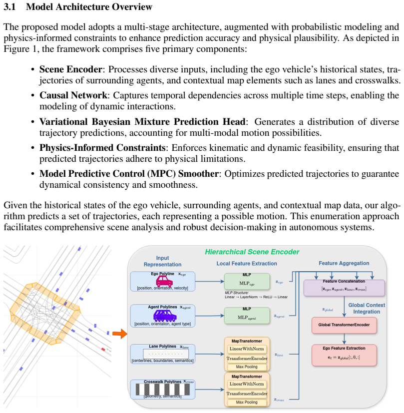
The load-bearing object is the variational Bayesian mixture prediction head. It outputs $K$ Gaussian components with means $\mu_k$, diagonal covariances $\Sigma_k$, and weights $\pi_k$, and it draws a latent variable $v\sim\mathcal{N}(\mu_v,\mathrm{diag}(\sigma_v^2))$ that is propagated through an LSTM over the future horizon before being folded into the per-mode predictions. The head sits inside a pipeline whose other components do specific work: the causal transformer enforces temporal causality, sector-boundary projection clamps points to a feasible radius and heading wedge, NMS sampling enforces endpoint diversity, and an MPC smoother with Ackermann dynamics solves an SLSQP optimization to produce dynamically consistent trajectories. The variational latent variable is what the paper uses to claim each mode represents a distribution of plausible futures instead of a single mean trajectory.
What would settle it
Inspect the training implementation and compute the gradient of the position loss with respect to the network parameters at initialization on a single batch. If it is exactly zero whenever the SLSQP solver is treated as a fixed operator, then the claimed end-to-end training through MPC smoothing does not occur, and the position loss cannot be responsible for the reported gains.
Extended reading notes
Core claim
The central claim is that representing the predictive distribution as $p(y|h)=\int p(y|v,h)p(v|h)\,dv$, with $v$ sampled from a diagonal Gaussian whose parameters are produced by an LSTM and propagated across the prediction horizon, gives each of the $K$ Gaussian mixture components an internal structure that captures variation within a mode. The paper further claims that this probabilistic head, embedded between a causal transformer and a refinement stage of sector-boundary projection, NMS sampling, and MPC smoothing, yields superior closed-loop performance on Lyft and nuPlan: for example, nuPlan collision rate drops to $6.83\%$ and off-road rate to $1.26\%$, below the reported CCIL numbers of $9.34\%$ and $5.58\%$. The stated upshot is that data-driven diversity and physical feasibility are complementary rather than in tension.
Load-bearing premise
The training loop assumes the position and yaw mistakes made after MPC smoothing can be fed back to improve the prediction network; the paper never states how that feedback passes through the numerical optimizer, and if the path is blocked the network cannot be trained as described.
Editorial extensions
If this is right
- A single 2.5M-parameter model can outperform substantially larger or deterministic baselines on closed-loop collision, off-road, discomfort, and L2 metrics on both Lyft and nuPlan.
- The variational latent variable turns each mixture component into a distribution over similar futures, so sampling can generate multiple trajectories per mode rather than one per anchor.
- Sector-boundary projection and MPC smoothing keep predictions kinematically feasible, which the paper argues makes them directly usable by downstream planners.
- Causal masking prevents future information leakage and is reported to matter especially in interactive scenarios.
- NMS sampling promotes endpoint diversity and reduces redundant trajectory hypotheses.
Reading between the lines
- The authors do not ablate the latent variable $v$ while keeping the same mixture head, so the paper's signature variational claim is not directly isolated; an ablation comparing $p(y|h)=\sum_k\pi_k\mathcal{N}(y|\mu_k,\Sigma_k)$ with and without $v$ would test it.
- The MPC smoother may contribute to the reported closed-loop gains as a post-processing safety filter; reporting raw predictions before sector projection and MPC would separate filtering from representation learning.
- The same architecture could be evaluated on open-loop metrics such as minADE and minFDE to test whether the closed-loop superiority transfers to direct prediction accuracy.
Editorial analysis
A structured set of objections, weighed in public.
Referee Report
Summary. The paper proposes PhysVarMix, a trajectory prediction system that combines a hierarchical scene encoder, a causal transformer, a mixture-of-Gaussians prediction head, sector-based physical constraints, NMS-based trajectory sampling, and an MPC smoother. The central methodological claim is that a latent variable v makes the prediction head a variational Bayesian mixture model that captures intra-mode variation, and the paper reports strong closed-loop results on Lyft and nuPlan, together with ablations and a small simulated experiment. The manuscript also provides a public repository link.
Significance. If the claims were supported, the paper would offer a useful hybrid baseline: it combines established encoders with post-hoc physics constraints and smoothing, and the experimental apparatus (two benchmarks, ablations, a simulated sanity check, and shared code) is a reasonable engineering contribution. However, the paper's stated novelty—the variational mixture mechanism—is not realized in the equations, and a second load-bearing training issue is unresolved. As written, the contribution reduces to a standard mixture density network with post-processing, so the significance of the claimed mechanism is not established.
major comments (3)
- [Section 3.7 / Appendix D.6] The latent variable v is never used to compute the mixture parameters. Equation (3.4) writes p(y|h) = ∫ p(y|v,h) p(v|h) dv, but Appendix D.3.1 defines the means and variances as linear functions of o_t only (vec(M_µ) = W_µ o_t + b_µ, vec(log M_σ2) = W_σ o_t + b_σ), and D.3.3 defines the mixture weights as π = MLP_π(o_t). The trajectory sampling and refinement in D.4 sample from N(µ_k, Σ_k) and never consume v_seq from D.3.2. Consequently p(y|v,h) = p(y|h), the integral collapses, and no intra-mode variation is captured. The only KL term in Section 3.7 is D_KL(Cat(π) || Uniform(K)), not a KL between q(v|h) and a prior, so no variational objective is optimized. The central variational claim is therefore not supported by the described forward model.
- [Section 4.3 / Table 1] The position loss L_pos is computed on the MPC-smoothed trajectories, but the MPC solve uses an SLSQP optimizer, which is not differentiable. The paper never states whether gradients flow through the optimizer, whether the MPC is approximated by a differentiable surrogate, or whether L_pos is treated as a fixed operator with an alternative training signal reaching the network. Without one of these mechanisms, the statement that parameters are updated via ∇_θ L_total using AdamW is not implementable as written. This is load-bearing because L_pos is the primary position loss and the paper gives no other route for the position error to affect the prediction head.
- [Section 4.3 / Table 1] The closed-loop evaluation protocol is not described. The paper does not state which closed-loop simulator is used for Lyft and nuPlan, which scenario sets are used, or how the deterministic baselines (Raster-perturb, BC-perturb, UrbanDriver) were executed in the same setting. Without this information, the cross-method comparisons in Table 1 cannot be reproduced or checked, and the very large improvements over prior baselines are difficult to interpret.
minor comments (6)
- [Table 1] The value for PhysVarMix on Lyft Collision is printed as '3,14' rather than '3.14'; this typo should be corrected.
- [Section 3.4 and Appendix D.3] The notation switches from h in Section 3.4 to o_t in Appendix D.3 without explicit identification; this makes it harder to trace whether v_seq is used anywhere.
- [Section 4.4, Table 2] Observation 2 says NMS sampling 'enhances the off-road navigation rate', but Table 2 shows off-road increasing from 0.73 without NMS to 0.81 with NMS; the wording should be clarified.
- [Table 2] The first three rows have 'Data.Std' and 'Ego' columns that are not clearly defined; in particular, the header 'Ego Collision (%)' appears to combine a flag and a metric, and the meaning of the checkmark in the Ego column is unexplained.
- [Table 3] The hyperparameter 'Auxiliary weight μ 0.3' is listed, but no auxiliary loss is defined in Section 3.7; please either define the loss or remove the entry.
- [Section 3.6 and Appendix A] The vehicle model in Section 3.6 is a nine-state Ackermann model, while Appendix A derives a simpler kinematic bicycle model; the discrepancy should be reconciled, as the MPC constraints depend on which model is actually used.
Circularity Check
The central variational latent variable is not connected to the predicted mixture, so Eq. 3.4's integral collapses to a standard Gaussian mixture head.
-
self definitional
[Section 3.4 (Variational Mixture Prediction Head), with Appendix D.3.2 and D.4.2]
"To further enhance the expressiveness of the model, we introduce a latent variable v ∈ RDlatent, which captures additional variations within each mode. The overall predictive distribution is formulated as: p(y|h) = ∫ p(y|v, h) p(v|h) dv ... Finally, the mixture parameters are computed by dedicated prediction heads as follows: µ1:K = Linearµ(h), σ1:K = exp(Linearσ(h)), π = Softmax(MLPπ(h))"
The GMM parameters µ, σ, and π are functions of h only. Nowhere does the paper define a conditional likelihood p(y|v,h) that depends on v; Appendix D.4.2 samples candidates from N(µk[t,:], diag(σ²k[t,:])) and the NMS/MPC stages never consume vseq. Hence p(y|v,h) = p(y|h) as a distribution over y, and the integral in Eq. 3.4 reduces to p(y|h) by construction. The claimed 'additional variations within each mode' are therefore not captured by the latent variable; the variational mixture derivation is mathematically identical to a standard mixture-of-Gaussians head with an unused random input.
-
other
[Section 3.7 (Loss Function) and Appendix D.6]
"LKL = 1/B Σ_b DKL(Cat(π_b) || Uniform(K)) is the KL divergence between mixture weights and a uniform distribution ... Parameters are updated via ∇θLtotal using AdamW."
This is the only KL term in the objective, and it regularizes the categorical mixture weights toward uniform; there is no KL divergence between an approximate posterior q(v|h) and a prior p(v|h), and no ELBO over the latent variable appears. Thus the 'variational' step in the derivation is not an optimized variational objective: the latent variable contributes no training signal and no density term, reinforcing that the variational claim is defined by equations that do not involve v.
full rationale
The benchmark claims (Table 1) are evaluated against external Lyft/nuPlan metrics, and no load-bearing self-citation chain appears: the cited works are unrelated external methods. However, the paper's central methodological novelty is the variational Bayesian mixture model with a latent variable v 'capturing additional variations within each mode.' By the paper's own equations, the mixture parameters µ1:K, σ1:K, and π are computed from h alone, the sampling/refinement stages never consume v (Appendix D.4.2 uses only µk and σk), and the only KL loss is over the categorical mixture weights, not over v. Therefore p(y|v,h) is independent of v, the integral in Section 3.4 collapses to p(y|h), and the 'variational latent variable' component reduces by construction to a conventional mixture-density head. This is a partial circularity: one central claimed component is vacuous, even though the MPC smoothing, NMS sampling, and external benchmark evaluation are not circular.
Assumptions & free parameters
free parameters (8)
- augmentation_std =
2
- num_mixtures_K =
6
- latent_dim =
16
- nms_distance_threshold =
1.4
- sector_boundary_radius =
10.0
- sector_boundary_angle =
pi/4
- mpc_weight_matrices =
Q and R as listed in Appendix C
- loss_weights =
yaw 0.3, uncertainty 0.1, KL 0.01
assumptions (6)
- domain assumption The Ackermann kinematic model with the stated dynamics is an adequate representation of vehicle motion for prediction and planning (Section 3.6, Appendix A).
- domain assumption The closed-loop simulator provides a fair and transferable evaluation of planning performance, and results generalize to real driving.
- ad hoc to paper Gradients of the position loss with respect to the network parameters can be obtained through the SLSQP-based MPC optimization, or the optimization is treated as a fixed non-differentiable operator with an alternative training signal.
- ad hoc to paper The latent variable v is drawn from a Gaussian and propagated through an LSTM, and this procedure is meant to capture intra-mode variation.
- domain assumption The CCIL baseline re-implemented by the authors from the paper description is a faithful reproduction.
- standard math Standard attention and MLP components function as described; no special theoretical guarantees are needed.
invented entities (1)
-
Latent variable v
Cite this review
Pith. "Pith review of PhysVarMix: Physics-Informed Variational Mixture Model for Multi-Modal Trajectory Prediction." pith.science (2026). https://pith.science/paper/3ZFIGWH5
@misc{pith2026250719701,
  author       = {Pith},
  title        = {Pith review of: PhysVarMix: Physics-Informed Variational Mixture Model for Multi-Modal Trajectory Prediction},
  year         = {2026},
  howpublished = {\url{https://pith.science/paper/3ZFIGWH5}},
  note         = {Machine review of arXiv:2507.19701}
}
read the original abstract
Accurate prediction of future agent trajectories is a critical challenge for ensuring safe and efficient autonomous navigation, particularly in complex urban environments characterized by multiple plausible future scenarios. In this paper, we present a novel hybrid approach that integrates learning-based with physics-based constraints to address the multi-modality inherent in trajectory prediction. Our method employs a variational Bayesian mixture model to effectively capture the diverse range of potential future behaviors, moving beyond traditional unimodal assumptions. Unlike prior approaches that predominantly treat trajectory prediction as a data-driven regression task, our framework incorporates physical realism through sector-specific boundary conditions and Model Predictive Control (MPC)-based smoothing. These constraints ensure that predicted trajectories are not only data-consistent but also physically plausible, adhering to kinematic and dynamic principles. Furthermore, our method produces interpretable and diverse trajectory predictions, enabling enhanced downstream decision-making and planning in autonomous driving systems. We evaluate our approach on two benchmark datasets, demonstrating superior performance compared to existing methods. Comprehensive ablation studies validate the contributions of each component and highlight their synergistic impact on prediction accuracy and reliability. By balancing data-driven insights with physics-informed constraints, our approach offers a robust and scalable solution for navigating the uncertainties of real-world urban environments.
Figures


Figures from the paper (4 more)


Reference graph
Works this paper leans on
-
[1]
I. Bae, J. Lee, and H.-G. Jeon. Can language beat numerical regression? language-based multimodal trajectory prediction, 2024
work page 2024
- [2]
-
[3]
C. M. Bishop. Mixture density networks. Technical report, Aston University, 1994
work page 1994
-
[4]
H. Caesar, J. Kabzan, K. S. Tan, W. K. Fong, E. Wolff, A. Lang, L. Fletcher, O. Beijbom, and S. Omari. nuplan: A closed-loop ml-based planning benchmark for autonomous vehicles. In 2021 IEEE/CVF Conference on Computer Vision and Pattern Recognition Workshops (CVPRW), pages 4237–4246. IEEE, June 2021
work page 2021
-
[5]
Y . Chai, B. Sapp, M. Bansal, and D. Anguelov. Multipath: Multiple probabilistic anchor trajectory hypotheses for behavior prediction. arXiv preprint arXiv:1910.05449, 2019
arXiv 1910
-
[6]
J. Chen, H. Zhang, Y . Li, and J. Sun. Learning map representations for autonomous driving: A survey. IEEE Transactions on Intelligent V ehicles, 7(4):891–905, December 2022
work page 2022
-
[7]
H. Cui, V . Radosavljevic, F.-C. Chou, T.-H. Lin, T. Nguyen, T.-K. Huang, J. Schneider, and N. Djuric. Multimodal trajectory predictions for autonomous driving using deep convolutional networks. arXiv preprint arXiv:1809.10732, 2018
arXiv 2018
-
[8]
P. Falcone, F. Borrelli, J. Asgari, H. E. Tseng, and D. Hrovat. Predictive active steering control for autonomous vehicle systems. IEEE Transactions on Control Systems Technology, 15(3):566–580, May 2007
work page 2007
Show all 49 references
-
[9]
Fujimoto and S
S. Fujimoto and S. S. Gu. A minimalist approach to offline reinforcement learn- ing. In Advances in Neural Information Processing Systems 34 (NeurIPS 2021) , vol- ume 34, pages 20132–20145. Curran Associates, Inc., December 2021. Available at: https://papers.nips.cc/paper/2021...
2021
-
[10]
X. Gao, X. Gao, J. Zhao, H. Wu, Z. Liu, and M. Li. Intention-aware denoising diffusion model for trajectory prediction, 2024
2024
-
[11]
Gilles, S
T. Gilles, S. Sabatini, D. Tsishkou, B. Stanciulescu, and F. Moutarde. Probabilistic multi- modal trajectory prediction with lane attention for autonomous vehicles. In 2021 IEEE/RSJ International Conference on Intelligent Robots and Systems (IROS) , pages 1428–1434. IEEE, Sept...
2021
-
[12]
Girgis, F
R. Girgis, F. Golemo, F. Codevilla, M. Weiss, S. D’Souza, S. E. Kahou, F. Heide, and C. Pal. La- tent variable sequential set transformers for joint multi-agent motion prediction. InInternational Conference on Learning Representations, 2022
2022
-
[13]
Gomes and D
I. Gomes and D. Wolf. A review on intention-aware and interaction-aware trajectory prediction for autonomous vehicles. In 2022 Latin American Robotics Symposium (LARS), 2022 Brazilian Symposium on Robotics (SBR), and 2022 Workshop on Robotics in Education (WRE) , pages 84–89. ...
2022
-
[14]
K. Guo, W. Jing, J. Chen, and J. Pan. Ccil: Context-conditioned imitation learning for urban driving, 2023
2023
-
[15]
A. Hari, Z. Liu, and R. Mangharam. Navigation under uncertainty: trajectory prediction and occlusion reasoning with switching dynamical systems, 2024
2024
-
[16]
K. He, X. Zhang, S. Ren, and J. Sun. Deep residual learning for image recognition. In 2016 IEEE Conference on Computer Vision and Pattern Recognition (CVPR) , pages 770–778. IEEE, June 2016. 19
2016
-
[17]
Hochreiter and J
S. Hochreiter and J. Schmidhuber. Long short-term memory. Neural Computation, 9(8):1735– 1780, 1997
1997
-
[18]
Houston, G
J. Houston, G. Zuidhof, L. Bergamini, Y . Ye, L. Chen, A. Jain, S. Omari, V . Iglovikov, and P. Ondruska. One thousand and one hours: Self-driving motion prediction dataset. In CoRL, 2020
2020
-
[19]
Huang, Y
Y . Huang, Y . Fan, X. Yang, B. Zhao, R. Yuan, R. Liu, Y . Zhang, and P. Li. A survey on trajectory- prediction methods for autonomous driving.IEEE Transactions on Intelligent V ehicles, 7(3):652– 674, September 2022
2022
-
[20]
Jeong, S
Y . Jeong, S. Lee, and K. Yi. Motion prediction of surrounding vehicles using deep neural networks for autonomous driving. In 2019 IEEE Intelligent V ehicles Symposium (IV), pages 1928–1933. IEEE, June 2019
2019
-
[21]
Karunakaran, J
D. Karunakaran, J. Yang, S. Fang, and W. Wang. Efficient prediction and uncertainty propagation for motion planning with multimodal behavior distribution. In 2023 IEEE 26th International Conference on Intelligent Transportation Systems (ITSC) , pages 3378–3385. IEEE, September 2023
2023
-
[22]
S. Kim, J. Lee, and H.-G. Jeon. Singulartrajectory: Universal trajectory predictor using diffusion model, 2024
2024
-
[23]
N. Lee, W. Choi, P. Vernaza, C. B. Choy, P. H. Torr, and M. Chandraker. Desire: Distant future prediction in dynamic scenes with interacting agents. In Proceedings of the IEEE Conference on Computer Vision and Pattern Recognition, pages 300–309, 2017
2017
-
[24]
Lefèvre, D
S. Lefèvre, D. Vasquez, and C. Laugier. A survey on motion prediction and risk assessment for intelligent vehicles. Robomech Journal, 1(1):1–14, 2014
2014
-
[25]
Z. Leng, H. Wang, S. Han, Y . Xing, K. Tang, J. Zhu, and Z. Xing. Traj-llm: A new exploration for empowering trajectory prediction with pre-trained large language models, 2024
2024
-
[26]
Leon and M
F. Leon and M. Gavrilescu. A review of tracking and trajectory prediction methods for au- tonomous driving. Mathematics, 9(6):660, March 2021
2021
-
[27]
J. Li, X. Tao, Y . Guo, and J. Lu. Spatio-temporal trajectory prediction with graph neural networks for autonomous driving. IEEE Transactions on V ehicular Technology, 70(8):7666–7678, August 2021
2021
-
[28]
Li and D
Z. Li and D. Pfoser. Hybrid machine learning model with a constrained action space for trajectory prediction, 2025
2025
-
[29]
Liang, B
M. Liang, B. Yang, R. Hu, Y . Chen, R. Liao, S. Feng, and R. Urtasun. Learning lane graph representations for motion forecasting. In European Conference on Computer Vision, pages 541–556. Springer, 2020
2020
-
[30]
Mercat, L
J. Mercat, L. Bartolo, J. Pettré, and N. L. Priol. Multi-head attention for multi-modal trajectory prediction in autonomous driving. In 2020 IEEE International Conference on Robotics and Automation (ICRA), pages 5688–5694. IEEE, May 2020
2020
-
[31]
Mozaffari, O
S. Mozaffari, O. Y . Al-Jarrah, M. Dianati, E. Moulas, and S. Fallah. Deep learning-based vehicle behavior prediction for autonomous driving applications: A review. IEEE Transactions on Intelligent Transportation Systems, 22(1):33–47, January 2021
2021
-
[32]
Mozaffari, E
S. Mozaffari, E. Arnold, M. Dianati, and S. Fallah. Multimodal maneuver prediction for autonomous vehicles using vehicular sensor and v2x data fusion. IEEE Transactions on Intelligent Transportation Systems, 23(12):23757–23770, December 2022
2022
-
[33]
Nayakanti, R
N. Nayakanti, R. Al-Rfou, A. Zhou, K. Goel, K. S. Refaat, and B. Sapp. Wayformer: Motion forecasting via simple & efficient attention networks. arXiv preprint arXiv:2207.05844, 2022
2022 arXiv
-
[34]
Ngiam, B
J. Ngiam, B. Caine, W. Han, B. Yang, Y . Chai, P. Lu, X. Peng, V . Vasudevan, X. Zhou, A. Chouard, et al. Scene transformer: A unified architecture for predicting multiple agent trajectories. arXiv preprint arXiv:2106.08417, 2021. 20
2021 arXiv
-
[35]
S. Ren, K. He, R. Girshick, and J. Sun. Faster r-cnn: Towards real-time object detection with region proposal networks. In Advances in neural information processing systems , pages 91–99, 2015
2015
-
[36]
Salzmann, B
T. Salzmann, B. Ivanovic, P. Chakravarty, and M. Pavone. Trajectron++: Dynamically-feasible trajectory forecasting with heterogeneous data. In 2020 European Conference on Computer Vision (ECCV), volume 12363 of Lecture Notes in Computer Science , pages 683–700. Springer, August 2020
2020
-
[38]
Schreier, V
M. Schreier, V . Willert, and J. Adamy. An integrated approach to maneuver-based trajectory prediction and criticality assessment in arbitrary road environments. In IEEE Transactions on Intelligent Transportation Systems, volume 17, pages 2751–2766. IEEE, October 2016
2016
-
[39]
K. Sohn, H. Lee, and X. Yan. Learning structured output representation using deep conditional generative models. In Advances in neural information processing systems , pages 3483–3491, 2015
2015
-
[40]
Sriramulu, N
A. Sriramulu, N. Fourrier, and C. Bergmeir. Multi-transmotion: Pre-trained model for human motion prediction, 2024
2024
-
[41]
R. Tumu, L. Lindemann, T. Nghiem, and R. Mangharam. Physics constrained motion prediction with uncertainty quantification, 2023
2023
-
[42]
Ulbrich, T
S. Ulbrich, T. Menzel, A. Reschka, F. Schuldt, and M. Maurer. Towards a functional system architecture for automated vehicles. In 2015 IEEE 18th International Conference on Intelligent Transportation Systems (ITSC), pages 1420–1425. IEEE, September 2015
2015
-
[43]
Vaswani, N
A. Vaswani, N. Shazeer, N. Parmar, J. Uszkoreit, L. Jones, A. N. Gomez, Ł. Kaiser, and I. Polosukhin. Attention is all you need. In Advances in neural information processing systems , pages 5998–6008, 2017
2017
-
[44]
Y . Wang, H. Wu, C. Liu, and C. Lv. A survey on deep learning-based autonomous driving: Methods and challenges. IEEE Transactions on Intelligent Transportation Systems, 24(5):4765– 4784, May 2023
2023
-
[45]
J. Xia, C. Xu, Y . Yan, Z. Fan, X. Gong, W. Huang, and F. Yu. Towards robust trajectory representations: Isolating environmental confounders with causal learning, 2024
2024
-
[46]
Yuan and K
Y . Yuan and K. Kitani. Dlow: Diversifying latent flows for diverse human motion prediction. In European Conference on Computer Vision, pages 346–364. Springer, 2020
2020
-
[47]
X. Zhao, H. Xiang, W. Yang, C. Feng, and J. Wang. A review of deep learning-based vehicle motion prediction for autonomous driving. IEEE Transactions on Intelligent Transportation Systems, 22(9):5667–5684, September 2021
2021
-
[48]
H. Zhou, H. Liu, Z. Zhang, Y . Xu, J. Yang, and J. Zhang. Smartpretrain: Model-agnostic and dataset-agnostic representation learning for motion prediction, 2024
2024
-
[49]
H. Zhou, Y . Xing, and C. Lv. Vectorized map representation for autonomous driving: A review. IEEE Transactions on Intelligent Transportation Systems, 24(7):6789–6804, July 2023. 21
2023
-
[2021]
Available at: https://arxiv.org/abs/2109.13333
Reviewed August 6, 2026 · model on record in the stance chip above.
Discussion (0). Sign in to comment.