A Weak Penalty Neural ODE for Learning Chaotic Dynamics from Noisy Time Series
Pith reviewed 2026-05-18 00:01 UTC · model grok-4.3
The pith
A weak formulation of the loss lets Neural ODEs filter noise and forecast chaotic dynamics accurately.
A machine-rendered reading of the paper's core claim, the machinery that carries it, and where it could break.
Core claim
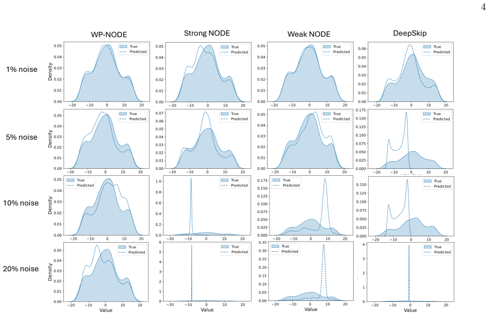
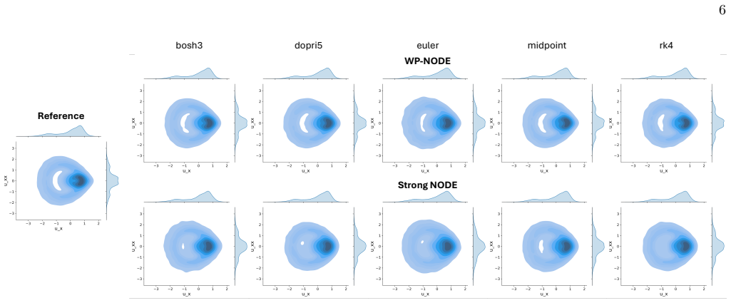
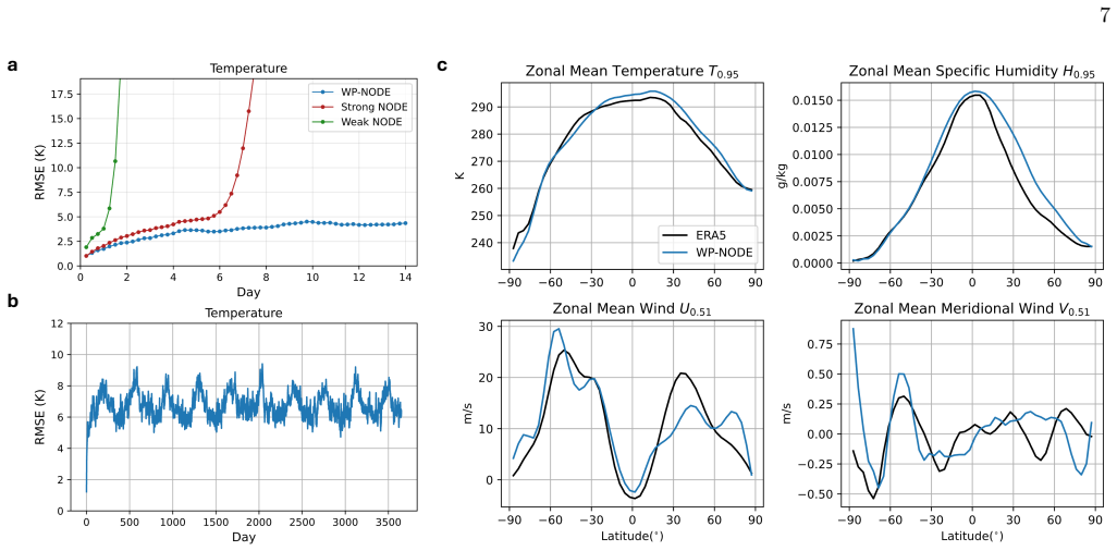
The authors show that the weak form of the Neural ODE residual, when used as a penalty in the training objective with suitable test functions and integration intervals, filters measurement noise in a manner equivalent to fitting the model to pre-filtered data. This formulation stabilizes training for chaotic attractors, where standard L2 losses on noisy trajectories lead to rapid divergence, and produces forecasts whose short-term accuracy and long-term invariants both improve. The method is demonstrated to be computationally efficient and independent of the particular ODE integrator chosen during training or prediction.
What carries the argument
The weak penalty loss, formed by integrating the Neural ODE residual against test functions over finite domains so that high-frequency noise contributions average toward zero.
If this is right
- The trained models achieve both short-term forecast accuracy and preservation of long-term invariant properties on standard chaotic benchmarks.
- The same strategy produces usable forecasts on a real-world climate dataset despite observational noise.
- Training remains efficient and works with any choice of numerical ODE solver.
- The approach avoids the exponential error growth that plagues standard Neural ODE training on noisy chaotic time series.
Where Pith is reading between the lines
- The same weak-penalty idea could be applied to other neural architectures that learn differential equations, such as neural SDEs or graph-based dynamical models.
- Optimal selection of test functions for a given noise spectrum or system dimension remains an open design choice that future work could automate.
- Because the method operates directly on the integral form, it may combine naturally with existing data-assimilation pipelines used in operational forecasting.
Load-bearing premise
The weak formulation with a proper choice of test function and integration domain effectively filters noisy data.
What would settle it
Train the model on a benchmark chaotic system with added noise, then verify whether the long-term statistics of simulated trajectories, such as the shape of the attractor or the leading Lyapunov exponent, match those obtained from clean data to within a small tolerance.
Figures


read the original abstract
The accurate forecasting of complex, high-dimensional dynamical systems from observational data is a fundamental task across numerous scientific and engineering disciplines. A significant challenge arises from noise-corrupted measurements, which severely degrade the performance of data-driven models. In chaotic dynamical systems, where small initial errors amplify exponentially, it is particularly difficult to develop a model from noisy data that achieves short-term accuracy while preserving long-term invariant properties. To overcome this, we consider the weak formulation as a complementary approach to the classical $L2$-loss function for training models of dynamical systems. We empirically verify that the weak formulation, with a proper choice of test function and integration domain, effectively filters noisy data. This insight explains why a weak form loss function is analogous to fitting a model to filtered data and provides a practical way to parameterize the weak form. Subsequently, we demonstrate how this approach overcomes the instability and inaccuracy of standard Neural ODE (NODE) in modeling chaotic systems. Through numerical examples, we show that our proposed training strategy, the Weak Penalty NODE, is computationally efficient, solver-agnostic, and yields accurate and robust forecasts across benchmark chaotic systems and a real-world climate dataset.
Editorial analysis
A structured set of objections, weighed in public.
Referee Report
Summary. The manuscript introduces the Weak Penalty Neural ODE (WP-NODE), which augments standard Neural ODE training with a weak-form loss term. The central claim is that, for a suitable choice of test function and integration domain, the weak formulation filters noise in time-series observations of chaotic systems, yielding short-term forecast accuracy while preserving long-term invariants; the method is further asserted to be computationally efficient and solver-agnostic, with supporting numerical results on benchmark chaotic systems and a real-world climate dataset.
Significance. If the noise-filtering property and long-term stability claims hold under broader conditions, the work would offer a practical, preprocessing-free route to training NODEs on noisy chaotic data. This could be useful in climate modeling and other domains where explicit denoising is costly or distorts invariants, and the solver-agnostic character would be a clear practical advantage.
major comments (2)
- [Abstract and weak-formulation section] Abstract and method description of the weak formulation: the assertion that 'the weak formulation, with a proper choice of test function and integration domain, effectively filters noisy data' is load-bearing for the entire approach, yet no general rule, stability analysis, or selection criterion is supplied for these choices. Without such guidance the reported success on the chosen benchmarks may reflect case-specific tuning rather than a structural guarantee, leaving the robustness claim for varying noise statistics or system dimensionality unproven.
- [Numerical experiments] Numerical experiments on long-term forecasts: while short-term accuracy and computational efficiency are shown, quantitative evidence that long-term invariants (e.g., Lyapunov exponents or attractor geometry) are preserved independently of the specific test-function parameters is limited. This weakens the claim that the method reliably overcomes standard NODE instability for chaotic systems.
minor comments (2)
- [Method] The notation used for the weak penalty loss should be contrasted explicitly with the classical L2 NODE loss to make the algorithmic difference immediately clear.
- [Numerical experiments] A short table or paragraph quantifying the sensitivity of forecast error to the integration-domain length would help readers assess practical implementation cost.
Simulated Author's Rebuttal
We thank the referee for their constructive and insightful comments. We address each major comment point by point below, indicating where revisions have been made to the manuscript.
read point-by-point responses
-
Referee: [Abstract and weak-formulation section] Abstract and method description of the weak formulation: the assertion that 'the weak formulation, with a proper choice of test function and integration domain, effectively filters noisy data' is load-bearing for the entire approach, yet no general rule, stability analysis, or selection criterion is supplied for these choices. Without such guidance the reported success on the chosen benchmarks may reflect case-specific tuning rather than a structural guarantee, leaving the robustness claim for varying noise statistics or system dimensionality unproven.
Authors: We appreciate this observation. The manuscript presents the approach as an empirical method and supplies a practical parameterization by showing that the weak-form loss corresponds to fitting filtered data, along with guidance on matching test-function support to system time scales (Section 3). We agree that more explicit selection criteria would improve clarity. In the revised manuscript we have added a dedicated paragraph in the method section that outlines concrete rules: choose the integration domain to exceed the noise correlation time but remain shorter than the system's Lyapunov time, and select test functions whose frequency content overlaps the dominant dynamics while attenuating high-frequency noise. A full stability analysis under arbitrary noise statistics and dimensionality is not derived, as it would require additional theoretical assumptions and development beyond the paper's empirical focus; robustness is instead demonstrated across multiple chaotic benchmarks with varying noise levels and dimensions. revision: partial
-
Referee: [Numerical experiments] Numerical experiments on long-term forecasts: while short-term accuracy and computational efficiency are shown, quantitative evidence that long-term invariants (e.g., Lyapunov exponents or attractor geometry) are preserved independently of the specific test-function parameters is limited. This weakens the claim that the method reliably overcomes standard NODE instability for chaotic systems.
Authors: We concur that stronger quantitative support for parameter independence would reinforce the long-term stability claim. The original experiments reported results for effective parameter choices. To address the concern, the revised manuscript now includes a sensitivity study: Lyapunov exponents and attractor geometry metrics (e.g., correlation dimension) are computed over a grid of test-function widths and integration lengths for each benchmark system. The results show that these invariants remain consistent within a practically useful range of parameters, with degradation only outside that range. Corresponding figures and tables have been added to the numerical experiments section. revision: yes
- A rigorous theoretical stability analysis of the weak formulation for arbitrary noise statistics and system dimensions is not provided.
Circularity Check
No significant circularity; method relies on empirical verification of weak-form filtering rather than self-referential derivation
full rationale
The paper presents the Weak Penalty NODE as a training strategy that leverages the weak formulation of dynamical systems to handle noisy data. The key assertion—that the weak form with suitable test functions and domains filters noise and is analogous to fitting filtered data—is stated as an empirical insight verified through numerical examples on benchmark chaotic systems and climate data. No load-bearing step reduces by construction to a fitted parameter renamed as prediction, a self-citation chain, or an ansatz smuggled via prior work. The derivation chain consists of proposing the penalty-augmented loss, demonstrating solver-agnostic training, and reporting forecast accuracy; these rest on external benchmarks and observed performance rather than tautological reparameterization of inputs. Self-contained against the provided numerical validation, this yields a normal non-finding of circularity.
Axiom & Free-Parameter Ledger
free parameters (1)
- test function and integration domain
axioms (1)
- domain assumption Weak formulation filters noisy data in dynamical systems when test functions and domains are chosen properly
Lean theorems connected to this paper
-
IndisputableMonolith/Cost/FunctionalEquation.leanwashburn_uniqueness_aczel unclear?
unclearRelation between the paper passage and the cited Recognition theorem.
the weak formulation, with a proper choice of test function and integration domain, effectively filters noisy data... L = L_weak + λ L_strong
-
IndisputableMonolith/Foundation/RealityFromDistinction.leanreality_from_one_distinction unclear?
unclearRelation between the paper passage and the cited Recognition theorem.
We empirically verify that the weak formulation... yields accurate and robust forecasts across benchmark chaotic systems
What do these tags mean?
- matches
- The paper's claim is directly supported by a theorem in the formal canon.
- supports
- The theorem supports part of the paper's argument, but the paper may add assumptions or extra steps.
- extends
- The paper goes beyond the formal theorem; the theorem is a base layer rather than the whole result.
- uses
- The paper appears to rely on the theorem as machinery.
- contradicts
- The paper's claim conflicts with a theorem or certificate in the canon.
- unclear
- Pith found a possible connection, but the passage is too broad, indirect, or ambiguous to say the theorem truly supports the claim.
Reference graph
Works this paper leans on
-
[1]
Evaluation is based on a validation threshold ofε= 0.3
In our numerical experiment, we integrate this system of ODEs using the RK4 scheme with a time step of ∆t= 0.01sfor 100s, yieldingN= 10 4 samples. Evaluation is based on a validation threshold ofε= 0.3. Under these parameters, the largest Lyapunov exponent is Λ≈0.91. First, 5% data noise is applied to the observation data, where a zero-mean Gaussian is de...
work page 2000
-
[2]
generalize residual networks by replacing discrete- layer architectures with a continuous-time dynamics model. Given an initial conditionu(t 0) =u 0, the evolu- tion of the state is governed by: du(t) dt =f(u(t), t;θ),(5) wherefis a neural network parameterized byθ. The so- lution at a later timetis determined by solving this initial value problem using s...
-
[3]
A. Ghadami and B. I. Epureanu, Data-driven prediction in dynamical systems: recent developments, Philosophi- cal Transactions of the Royal Society A380, 20210213 (2022)
work page 2022
-
[4]
F. Morrison,The art of modeling dynamic systems: fore- casting for chaos, randomness and determinism(Courier Corporation, 2012)
work page 2012
-
[5]
K. Kaheman, E. Kaiser, B. Strom, J. N. Kutz, and S. L. Brunton, Learning discrepancy models from experimen- tal data, arXiv preprint arXiv:1909.08574 (2019)
- [6]
-
[7]
S. L. Brunton and J. N. Kutz,Data-driven science and engineering: Machine learning, dynamical systems, and control(Cambridge University Press, 2022)
work page 2022
-
[8]
R. Wang, D. Maddix, C. Faloutsos, Y. Wang, and R. Yu, Bridging physics-based and data-driven modeling for learning dynamical systems, inLearning for dynamics and control(PMLR, 2021) pp. 385–398
work page 2021
-
[9]
D. Floryan and M. D. Graham, Data-driven discovery of intrinsic dynamics, Nature Machine Intelligence4, 1113 (2022)
work page 2022
-
[10]
M. J. Colbrook and A. Townsend, Rigorous data-driven computation of spectral properties of koopman operators for dynamical systems, Communications on Pure and Ap- plied Mathematics77, 221 (2024)
work page 2024
-
[11]
A. A. Kaptanoglu, J. L. Callaham, A. Aravkin, C. J. Hansen, and S. L. Brunton, Promoting global stability in data-driven models of quadratic nonlinear dynamics, Physical Review Fluids6, 094401 (2021)
work page 2021
-
[12]
C. Legaard, T. Schranz, G. Schweiger, J. Drgoˇ na, B. Falay, C. Gomes, A. Iosifidis, M. Abkar, and P. Larsen, Constructing neural network based models for simulat- ing dynamical systems, ACM Computing Surveys55, 1 (2023)
work page 2023
-
[13]
W. Gilpin, Chaos as an interpretable benchmark for forecasting and data-driven modelling, arXiv preprint arXiv:2110.05266 (2021)
-
[14]
M. Levine and A. Stuart, A framework for machine learning of model error in dynamical systems, Commu- nications of the American Mathematical Society2, 283 (2022)
work page 2022
-
[15]
D. E. Rumelhart, G. E. Hinton, and R. J. Williams, Learning representations by back-propagating errors, na- ture323, 533 (1986)
work page 1986
-
[16]
A. Chattopadhyay, P. Hassanzadeh, and D. Subrama- nian, Data-driven prediction of a multi-scale lorenz 96 chaotic system using deep learning methods: Reservoir computing, ann, and rnn-lstm, Nonlinear Processes in Geophysics Discussions2020, 1 (2020)
work page 2020
-
[17]
S. Hochreiter and J. Schmidhuber, Long short-term mem- ory, Neural computation9, 1735 (1997)
work page 1997
- [18]
-
[19]
M. U. Kobayashi, K. Nakai, Y. Saiki, and N. Tsutsumi, Dynamical system analysis of a data-driven model con- structed by reservoir computing, Physical Review E104, 044215 (2021)
work page 2021
-
[20]
M. Yan, C. Huang, P. Bienstman, P. Tino, W. Lin, and J. Sun, Emerging opportunities and challenges for the future of reservoir computing, Nature Communications 15, 2056 (2024)
work page 2056
-
[21]
F. M. Bianchi, S. Scardapane, S. Løkse, and R. Jenssen, Reservoir computing approaches for representation and classification of multivariate time series, IEEE transac- tions on neural networks and learning systems32, 2169 (2020)
work page 2020
-
[22]
C. Lea, R. Vidal, A. Reiter, and G. D. Hager, Tempo- ral convolutional networks: A unified approach to action segmentation, inEuropean conference on computer vision (Springer, 2016) pp. 47–54
work page 2016
-
[23]
V. Perumal, D. Abueidda, S. Koric, and A. Kontsos, Temporal convolutional networks for data-driven ther- mal modeling of directed energy deposition, Journal of Manufacturing Processes85, 405 (2023)
work page 2023
-
[24]
A. Vaswani, N. Shazeer, N. Parmar, J. Uszkoreit, L. Jones, A. N. Gomez, L. Kaiser, and I. Polosukhin, At- tention is all you need, Advances in neural information processing systems30(2017)
work page 2017
- [25]
- [26]
-
[27]
P. Mandal and G. A. Gottwald, Learning dynamical systems with hit-and-run random feature maps, Nature Communications16, 5961 (2025)
work page 2025
-
[28]
R. T. Chen, Y. Rubanova, J. Bettencourt, and D. K. Du- venaud, Neural ordinary differential equations, Advances in neural information processing systems31(2018)
work page 2018
- [29]
-
[30]
Kidger, On neural differential equations, arXiv preprint arXiv:2202.02435 (2022)
P. Kidger, On neural differential equations, arXiv preprint arXiv:2202.02435 (2022)
-
[31]
O. Ronneberger, P. Fischer, and T. Brox, U-net: Con- volutional networks for biomedical image segmentation, inInternational Conference on Medical image computing and computer-assisted intervention(Springer, 2015) pp. 234–241
work page 2015
-
[32]
Universal Differential Equations for Scientific Machine Learning
C. Rackauckas, Y. Ma, J. Martensen, C. Warner, K. Zubov, R. Supekar, D. Skinner, A. Ramadhan, and A. Edelman, Universal differential equations for scien- tific machine learning, arXiv preprint arXiv:2001.04385 (2020)
work page internal anchor Pith review arXiv 2001
-
[33]
Y. Ma, V. Dixit, M. J. Innes, X. Guo, and C. Rack- 11 auckas, A comparison of automatic differentiation and continuous sensitivity analysis for derivatives of differen- tial equation solutions, in2021 IEEE High Performance Extreme Computing Conference (HPEC)(IEEE, 2021) pp. 1–9
work page 2021
-
[34]
D. Chakraborty, S. W. Chung, T. Arcomano, and R. Maulik, Divide and conquer: Learning chaotic dy- namical systems with multistep penalty neural ordinary differential equations, Computer Methods in Applied Me- chanics and Engineering432, 117442 (2024)
work page 2024
-
[35]
D. Chakraborty, S. W. Chung, A. Chattopadhyay, and R. Maulik, Improved deep learning of chaotic dynami- cal systems with multistep penalty losses, arXiv preprint arXiv:2410.05572 (2024)
-
[36]
A. Allauzen, T. P. M. Dardis, and H. Plath, Exper- imental study of neural ode training with adaptive solver for dynamical systems modeling, arXiv preprint arXiv:2211.06972 (2022)
-
[37]
A. J. Linot, J. W. Burby, Q. Tang, P. Balaprakash, M. D. Graham, and R. Maulik, Stabilized neural ordinary dif- ferential equations for long-time forecasting of dynamical systems, Journal of Computational Physics474, 111838 (2023)
work page 2023
-
[38]
C. Fronk and L. Petzold, Training stiff neural ordinary differential equations with explicit rational taylor series methods, Chaos: An Interdisciplinary Journal of Nonlin- ear Science35(2025)
work page 2025
-
[39]
C. Fronk and L. Petzold, Training stiff neural ordinary differential equations with implicit single-step methods, Chaos: An Interdisciplinary Journal of Nonlinear Science 34(2024)
work page 2024
-
[40]
S. Cheng, C. Quilodr´ an-Casas, S. Ouala, A. Farchi, C. Liu, P. Tandeo, R. Fablet, D. Lucor, B. Iooss, J. Bra- jard,et al., Machine learning with data assimilation and uncertainty quantification for dynamical systems: a re- view, IEEE/CAA Journal of Automatica Sinica10, 1361 (2023)
work page 2023
-
[41]
S. Mukhopadhyay and S. Banerjee, Learning dynami- cal systems in noise using convolutional neural networks, Chaos: An Interdisciplinary Journal of Nonlinear Science 30(2020)
work page 2020
-
[42]
D. A. Messenger and D. M. Bortz, Weak sindy for partial differential equations, Journal of Computational Physics 443, 110525 (2021)
work page 2021
-
[43]
J. Hsin, S. Agarwal, A. Thorpe, L. Sentis, and D. Fridovich-Keil, Symbolic regression on sparse and noisy data with gaussian processes, in2025 American Control Conference (ACC)(IEEE, 2025) pp. 3170–3175
work page 2025
-
[44]
S. Yang, S. W. Wong, and S. Kou, Inference of dy- namic systems from noisy and sparse data via manifold- constrained gaussian processes, Proceedings of the Na- tional Academy of Sciences118, e2020397118 (2021)
work page 2021
- [45]
-
[46]
A. Seleznev, D. Mukhin, A. Gavrilov, E. Loskutov, and A. Feigin, Bayesian framework for simulation of dynam- ical systems from multidimensional data using recurrent neural network, Chaos: An Interdisciplinary Journal of Nonlinear Science29(2019)
work page 2019
-
[47]
L. Yang, X. Meng, and G. E. Karniadakis, B-pinns: Bayesian physics-informed neural networks for forward and inverse pde problems with noisy data, Journal of Computational Physics425, 109913 (2021)
work page 2021
- [48]
-
[49]
L. Ding and C. Wen, High-order extended kalman filter for state estimation of nonlinear systems, Symmetry16, 617 (2024)
work page 2024
-
[50]
R. Stephany and C. Earls, Weak-pde-learn: A weak form based approach to discovering pdes from noisy, lim- ited data, Journal of Computational Physics506, 112950 (2024)
work page 2024
-
[51]
D. M. Bortz, D. A. Messenger, and A. Tran, Weak form- based data-driven modeling: Computationally efficient and noise robust equation learning and parameter infer- ence, inHandbook of Numerical Analysis, Vol. 25 (Else- vier, 2024) pp. 53–82
work page 2024
- [52]
-
[53]
T. De Ryck, S. Mishra, and R. Molinaro, wpinns: Weak physics informed neural networks for approximating en- tropy solutions of hyperbolic conservation laws, SIAM Journal on Numerical Analysis62, 811 (2024)
work page 2024
-
[54]
E. Kharazmi, Z. Zhang, and G. E. Karniadakis, hp- vpinns: Variational physics-informed neural networks with domain decomposition, Computer Methods in Ap- plied Mechanics and Engineering374, 113547 (2021)
work page 2021
-
[55]
D. A. Messenger and D. M. Bortz, Weak sindy: Galerkin- based data-driven model selection, Multiscale Modeling & Simulation19, 1474 (2021)
work page 2021
-
[56]
H. Zhao, Y. Wang, H. Qi, Z. Huang, H. Zhao, L. Sha, and H. Shao, Accelerating neural odes: A variational formulation-based approach, inThe Thirteenth Interna- tional Conference on Learning Representations(2025)
work page 2025
-
[57]
S. Kullback and R. A. Leibler, On information and suf- ficiency, The annals of mathematical statistics22, 79 (1951)
work page 1951
-
[58]
E. N. Lorenz, Deterministic nonperiodic flow 1, inUni- versality in Chaos, 2nd edition(Routledge, 2017) pp. 367–378
work page 2017
-
[59]
E. N. Lorenz, Predictability: A problem partly solved, in Proc. Seminar on predictability, Vol. 1 (Readinhig, 1996) pp. 1–18
work page 1996
-
[60]
R. A. Edson, J. E. Bunder, T. W. Mattner, and A. J. Roberts, Lyapunov exponents of the kuramoto– sivashinsky pde, The ANZIAM Journal61, 270 (2019)
work page 2019
-
[61]
H. Fan, J. Jiang, C. Zhang, X. Wang, and Y.-C. Lai, Long-term prediction of chaotic systems with machine learning, Physical Review Research2, 012080 (2020)
work page 2020
-
[62]
H. Hersbach, B. Bell, P. Berrisford, S. Hirahara, A. Hor´ anyi, J. Mu˜ noz-Sabater, J. Nicolas, C. Peubey, R. Radu, D. Schepers,et al., The era5 global reanaly- sis, Quarterly journal of the royal meteorological society 146, 1999 (2020)
work page 1999
-
[63]
T. Arcomano, I. Szunyogh, A. Wikner, J. Pathak, B. R. Hunt, and E. Ott, A hybrid approach to atmospheric modeling that combines machine learning with a physics- based numerical model, Journal of Advances in Modeling Earth Systems14, e2021MS002712 (2022)
work page 2022
- [64]
-
[65]
J. R. Dormand and P. J. Prince, A family of embedded runge-kutta formulae, Journal of computational and ap- plied mathematics6, 19 (1980)
work page 1980
-
[66]
J. C. Butcher,Numerical methods for ordinary differen- tial equations(John Wiley & Sons, 2016). 13 Supplementary Information SUPPLEMENT AR Y NOTE 1: LORENZ 63 INV ARIANT MEASURE ANAL YSIS To complement the quantitative KL divergence results presented in Table 1 of the article, this note provides a detailed visual comparison of the predicted and ground-tru...
work page 2016
-
[67]
Linear Basis Functions.Define the piecewise linear Lagrange basis functionsℓ i(s), ℓi(s) = s−s i−1 si −s i−1 , s∈[s i−1, si] si+1 −s si+1 −s i , s∈[s i, si+1] 0,otherwise for 1≤i≤M−2. For the endpoints: ℓ0(s) = s1 −s s1 −s 0 , s∈[s 0, s1] 0,otherwise ℓM−1(s) = s−s M−2 sM−1 −s M−2 , s∈[s M−2 , sM−1] 0,otherwise
-
[68]
Interpolant Construction.We define the linear interpolants of the functionsx(s) andf(u(s), s;θ) as: ˜x(s) = M−1X i=0 xiℓi(s), ˜f(s) = M−1X i=0 fiℓi(s).(S2) These functions are continuous and piecewise linear. Note that ifx i, fi ∈R D are vectors andℓ i(s)∈Ris a scalar, the termsx iℓi(s) andf iℓi(s) represent the standard scalar-vector products
-
[69]
Projection Against a Test Function.We approximate the following integrals using Eq. (S2) as follows, L 2 Z sM−1 s0 f(x(s), s;θ)ϕ(s)ds≈ L 2 Z sM−1 s0 ˜f(s)ϕ(s)ds= M−1X i=0 fi L 2 Z sM−1 s0 ℓi(s)ϕ(s)ds = M−1X i=0 fiwrhs,i, where the weights are defined as: wrhs,i = L 2 Z sM−1 s0 ℓi(s)ϕ(s)ds. 22 Similarly, Z sM−1 s0 x(s)ϕ′(s)ds≈ Z sM−1 s0 ˜x(s)ϕ′(s)ds= M−1X ...
-
[70]
Explicit Expression for Weights.For interior indices 1≤i≤M−2, we have: wrhs,i = L 2 Z si si−1 s−s i−1 si −s i−1 ϕ(s)ds+ L 2 Z si+1 si si+1 −s si+1 −s i ϕ(s)ds = L 2(si −s i−1) [Ψ(si)−Ψ(s i−1)−s i−1(Φ(si)−Φ(s i−1))] + L 2(si+1 −s i) [si+1(Φ(si+1)−Φ(s i))−Ψ(s i+1) + Ψ(si)], where Φp,d(s) = R ϕ(d) p (s)dsand Ψ p,d(s) = R sϕ(d) p (s)ds. For the endpoints: wrh...
work page 2048
discussion (0)
Sign in with ORCID, Apple, or X to comment. Anyone can read and Pith papers without signing in.