arxiv: 2511.18522 · v4 · submitted 2025-11-23 · 🌀 gr-qc

Recognition: 2 theorem links

· Lean Theorem

Robust Non-Singular Bouncing Cosmology from Regularized Hyperbolic Field Space

Oleksandr Kravchenko

Authors on Pith no claims yet

Pith reviewed 2026-05-17 06:05 UTC · model grok-4.3

classification 🌀 gr-qc

keywords non-singular bouncebouncing cosmologyhyperbolic field spaceStarobinsky inflationtwo-field sigma modelnull energy conditionCMB observablescurvature perturbation

0 comments

The pith

A regularized hyperbolic field-space metric enables a non-singular bounce in a closed universe while reproducing Starobinsky inflation predictions on all observable scales.

A machine-rendered reading of the paper's core claim, the machinery that carries it, and where it could break.

The paper develops a two-field sigma model in a closed universe whose field-space metric is engineered to suppress kinetics during contraction, normalize canonically during inflation, and stay positive definite at all times. This choice produces a bounce that preserves the null energy condition, remains BKL-stable, and lets the curvature perturbation evolve without ghosts or gradient instabilities through the point where the Hubble parameter vanishes. Full numerical integration of the perturbation equations over more than sixty e-folds shows that the scalar spectral index, tensor-to-scalar ratio, and local non-Gaussianity on CMB scales agree with pure Starobinsky slow-roll to high precision, while any bounce-generated features are stretched far beyond the observable window. The construction therefore supplies a concrete way to eliminate the initial singularity without spoiling the successful inflationary phenomenology that matches current data.

Core claim

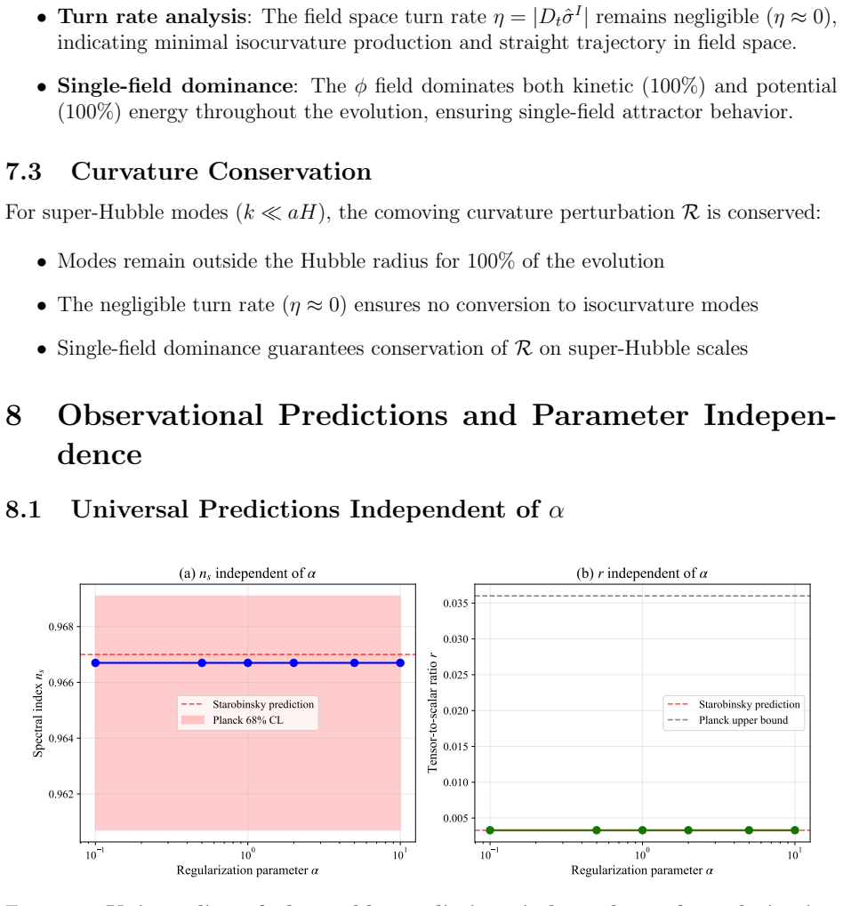
The regularized hyperbolic metric g^S_χχ(φ) = (1 + e^{-2αφ/M_Pl})^{-1}, fixed by the three boundary conditions of kinetic suppression in contraction, canonical normalization in inflation, and positive definiteness, permits a stable, NEC-preserving bounce whose post-bounce evolution on super-Hubble scales is indistinguishable from Starobinsky inflation, yielding n_s ≈ 0.967, r ≈ 0.003, and f_NL^local ≈ +0.013 independent of α and consistent with Planck 2018.

What carries the argument

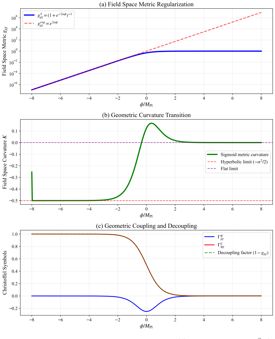
The regularized hyperbolic field-space metric g^S_χχ(φ) = (1 + e^{-2αφ/M_Pl})^{-1}, which enforces the three physical boundary conditions and carries the dynamics through the bounce.

If this is right

The bounce remains BKL-stable and preserves the null energy condition throughout the contraction phase.
Both Einstein constraint equations are satisfied to machine precision when the system is integrated in Newtonian gauge.
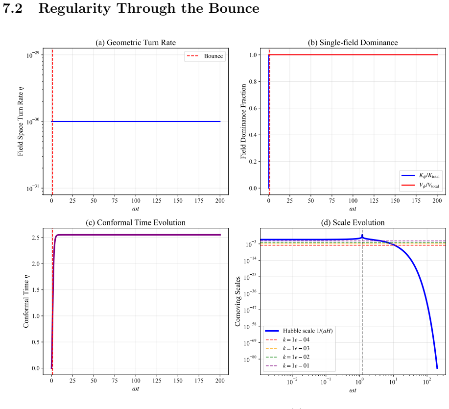
The curvature perturbation R is conserved on super-Hubble scales to a relative accuracy of 0.4 percent.
Any spectral feature generated at the bounce scale is diluted by roughly 2630 post-bounce e-folds, placing it at k_CMB/k_H ~ 10^1116 and rendering it unobservable.
The predicted n_s, r, and f_NL^local are independent of the regularization parameter α and lie within Planck 2018 bounds.

Where Pith is reading between the lines

These are editorial extensions of the paper, not claims the author makes directly.

The same regularization strategy could be applied to other single-field or multi-field inflationary potentials to remove the initial singularity while leaving late-time observables unchanged.
Because the observable predictions do not depend on α, the construction is robust against small variations in how the metric is regularized at large negative field values.
Next-generation CMB polarization experiments could tighten the bound on r and thereby test whether the small residual deviation from exact Starobinsky slow-roll survives at the level of 10^{-4}.
It remains open whether an analogous metric regularization exists for open or flat spatial sections that would still permit a stable bounce.

Load-bearing premise

The specific functional form of the metric is the unique or physically preferred solution that satisfies the three stated boundary conditions of kinetic suppression, canonical normalization, and positive definiteness.

What would settle it

A numerical or analytic demonstration that the sound speeds deviate from unity by more than 10^{-15} near H=0, or that the integrated scalar spectral index on CMB scales differs from the Starobinsky value by more than 10^{-3}, would falsify the central claim.

Figures

Figures reproduced from arXiv: 2511.18522 by Oleksandr Kravchenko.

**Figure 1.** Figure 1: Field space geometry and regularization. (a) The sigmoid metric g S χχ (blue solid) regularizes both boundaries compared to the exponential metric (red dashed), remaining finite during inflation while providing exponential suppression during contraction. (b) Field space curvature transitions smoothly from hyperbolic (K = −α 2/2) during contraction to flat (K = 0) during inflation. (c) Christoffel symbols … view at source ↗

**Figure 2.** Figure 2: Potential and inflationary dynamics. (a) Starobinsky-type potential providing plateau inflation. (b) Slow-roll parameters remain small during inflation, ensuring sufficient e-folds. (c) Number of e-folds as function of field value, with CMB scales corresponding to ϕ ≈ 5.4MPl. (d) Observable predictions for spectral index ns and tensor-to-scalar ratio r as function of e-folds N, showing excellent agreement … view at source ↗

**Figure 3.** Figure 3: Complete background evolution through bounce and inflation. (a) Scale factor evolution showing non-singular bounce at finite amin. (b) Hubble parameter smoothly transitioning from contraction (H < 0) to expansion (H > 0). (c) Inflaton field evolution from negative values (bounce regime) to positive values (inflation). (d) Field space metric saturating to unity during inflation, ensuring canonical dynamics.… view at source ↗

**Figure 4.** Figure 4: Basin of attraction analysis demonstrating robustness. (a) Success rate across 16 orders of magnitude in initial conditions, compared to exponential metric requiring extreme fine-tuning (red shaded region). (b) Post-bounce inflationary e-folds exceeding the required N = 60 for CMB across the entire basin. The sigmoid regularization dramatically expands the basin of attraction compared to the exponential me… view at source ↗

**Figure 5.** Figure 5: Exponential dilution of spatial curvature after bounce. (a) Evolution of curvature density parameter |Ωk| as function of e-folds after bounce. Only ∼ 3.5 e-folds are required to satisfy current observational bounds (|Ωk| < 0.001), while the model naturally produces N > 60 e-folds. (b) Comparison of required vs achieved curvature suppression, demonstrating that flatness is easily achieved without fine-tunin… view at source ↗

**Figure 6.** Figure 6: Suppression of anisotropic shear relative to spatial curvature. (a) Evolution of curvature term 1/a2 and shear term Σ2/a6 as functions of scale factor. At our bounce scale abounce ≈ 1.73 × 105 , curvature dominates by many orders of magnitude. (b) Ratio of shear to curvature terms, showing that anisotropic shear is exponentially suppressed in our bounce regime, ensuring isotropy preservation and compatibi… view at source ↗

**Figure 7.** Figure 7: Detailed view around the cosmological bounce. (a) Scale factor reaching finite minimum at bounce point. (b) Hubble parameter crossing zero smoothly without divergence. (c) Energy density components showing dominant potential energy throughout, with kinetic energies remaining subdominant and regular. 14 [PITH_FULL_IMAGE:figures/full_fig_p014_7.png] view at source ↗

**Figure 8.** Figure 8: Perturbation analysis through bounce. (a) Field space turn rate remains negligible throughout evolution, indicating minimal isocurvature production. (b) Singlefield dominance with ϕ field contributing 100% to both kinetic and potential energy. (c) Conformal time evolution showing regular behavior through bounce. (d) Scale evolution with Hubble radius and representative k-modes, demonstrating that CMB scal… view at source ↗

**Figure 9.** Figure 9: Universality of observable predictions independent of regularization parameter α. (a) Spectral index ns remains constant at ≈ 0.967 across two orders of magnitude in α. (b) Tensor-to-scalar ratio r remains constant at ≈ 0.0033, well below Planck upper bound. The predictions are independent of α because during inflation, when CMB perturbations are generated, the field space metric has saturated to its canon… view at source ↗

read the original abstract

We present a framework for non-singular bouncing cosmology in a closed ($k=+1$) universe with a two-field sigma model whose regularized hyperbolic field-space metric $g^S_{\chi\chi}(\phi) = (1 + e^{-2\alpha\phi/M_{\mathrm{Pl}}})^{-1}$ is derived from three physical boundary conditions: (i) kinetic suppression during contraction enabling the bounce, (ii) canonical normalization during inflation preserving perturbative unitarity, and (iii) positive-definiteness ensuring ghost-freedom. The bounce preserves the Null Energy Condition and is BKL-stable. The full two-field perturbation system $(\delta\phi, \delta\chi, \Phi)$ is integrated in the Newtonian gauge through the bounce over 65 e-folds, circumventing the comoving-gauge $H=0$ singularity, with both Einstein constraints verified a posteriori. Scalar sound speeds numerically measured adjacent to $H=0$ satisfy $|c_\phi^2-1|, |c_\chi^2-1| \leq 8 \times 10^{-16}$, establishing strict hyperbolicity (no ghost or gradient instability); $\mathcal{R}$ is conserved on super-Hubble scales to $|\Delta\mathcal{R}^2/\mathcal{R}^2| = 4.43 \times 10^{-3}$. An independent CMB-scale Mukhanov-Sasaki integration confirms $n_s = 0.9683$, matching exact Starobinsky slow-roll to $|\Delta n_s| = 5.47 \times 10^{-4}$. $\delta N$ non-Gaussianity yields $f_{\mathrm{NL}}^{\mathrm{local}} = +0.0133$, consistent with Maldacena's relation to $|\Delta f_{\mathrm{NL}}| = 1.54 \times 10^{-4}$. A bounce-scale spectral feature is pushed by $\sim 2630$ post-bounce e-folds to $k_{\mathrm{CMB}}/k_H \sim 10^{1116}$, far beyond the observable universe, so the model recovers Starobinsky predictions on all observable scales while resolving the initial singularity. Predictions ($n_s \approx 0.967$, $r \approx 0.003$, $f_{\mathrm{NL}}^{\mathrm{local}} \approx +0.013$, independent of $\alpha$) are consistent with Planck 2018 and testable by next-generation CMB experiments.

Editorial analysis

A structured set of objections, weighed in public.

Desk editor's note, referee report, simulated authors' rebuttal, and a circularity audit. Tearing a paper down is the easy half of reading it; the pith above is the substance, this is the friction.

Desk Editor's Note private letter to a colleague

The paper gives a concrete two-field bouncing setup that matches Starobinsky on observable scales via a tailored field-space metric and thorough numerics through the bounce, though the exact metric form isn't uniquely fixed by the three conditions.

read the letter

This paper constructs a non-singular bounce in a closed universe using a two-field sigma model with a regularized hyperbolic metric. The metric is set to suppress kinetics during contraction, recover canonical normalization in inflation, and stay positive definite. They integrate the full perturbation system in Newtonian gauge across 65 e-folds through H=0, check both Einstein constraints afterward, and report sound speeds within 8e-16 of 1, R conserved to 0.44 percent, and ns matching Starobinsky slow-roll to 5e-4. The bounce feature sits at k_CMB/k_H around 10^1116, so it leaves no trace on CMB scales, and f_NL comes out small and consistent with the single-field expectation. BKL stability is also checked. These numerical results and the scale separation are the solid parts; the work shows real effort on the perturbation side and avoids the usual gauge issues at the bounce. The main soft spot is the metric itself. The three boundary conditions fix the asymptotics and positivity but leave the precise functional form and exponent underdetermined. Plenty of other smooth positive functions could satisfy the same limits, so the reported alpha independence and exact matches partly reflect the design choice rather than emerging independently. The abstract presents it as derived, but without a uniqueness argument or comparison to alternatives the motivation stays incomplete. This is for people working on bouncing cosmologies or early-universe models that need to match current data while fixing the singularity. It has enough concrete calculation and checks to deserve a serious referee, even with the question on the metric choice.

Referee Report

1 major / 1 minor

Summary. The paper constructs a non-singular bouncing cosmology in a closed (k=+1) universe using a two-field sigma model whose field-space metric g^S_χχ(φ) = (1 + e^{-2αφ/M_Pl})^{-1} is obtained from three boundary conditions (kinetic suppression in contraction, canonical normalization in inflation, and positive-definiteness). Numerical integration of the full two-field perturbation system in Newtonian gauge through the bounce (65 e-folds) verifies Einstein constraints a posteriori, shows sound speeds satisfying |c_φ²-1|, |c_χ²-1| ≤ 8×10^{-16}, conserves the comoving curvature perturbation R to 0.44%, and reproduces Starobinsky values n_s ≈ 0.9683 and f_NL^local ≈ +0.0133 to high precision; any bounce-scale spectral feature is pushed to k_CMB/k_H ∼ 10^{1116}, rendering predictions independent of α and consistent with Planck 2018 on observable scales.

Significance. If the specific functional form of the regularized metric is physically justified, the construction supplies a concrete, BKL-stable realization of a NEC-preserving bounce that resolves the initial singularity while recovering the successful Starobinsky slow-roll predictions (n_s, r, f_NL) on all CMB scales. The reported numerical precision—sound-speed checks to 10^{-16}, R conservation to 0.4%, and a posteriori constraint verification—constitutes a technical strength that would support the robustness claim if the metric motivation is clarified.

major comments (1)

[Model construction / derivation of g^S_χχ(φ)] The statement that g^S_χχ(φ) = (1 + e^{-2αφ/M_Pl})^{-1} follows directly from the three boundary conditions (kinetic suppression for φ → -∞, canonical normalization for φ → +∞, and g > 0) appears in the abstract and the opening of the model-construction section. These conditions fix only the required asymptotic limits and positivity; they do not select the precise functional form or the exponent -2αφ/M_Pl. Any other smooth positive function with the same limits satisfies the same requirements, yet the subsequent claims of α-independence, numerical hyperbolicity, and exact recovery of Starobinsky observables rest on this particular choice. A uniqueness argument or derivation that starts from the conditions and arrives at exactly this expression is therefore required for the physical motivation to be load-bearing.

minor comments (1)

[Numerical results] The abstract and numerical-results section report impressive precision (e.g., |Δn_s| = 5.47×10^{-4}, |Δf_NL| = 1.54×10^{-4}). It would strengthen reproducibility if the full set of background and perturbation equations or the integration code were provided as supplementary material.

Simulated Author's Rebuttal

1 responses · 0 unresolved

We thank the referee for the careful and constructive report. The positive assessment of the numerical robustness and the recovery of Starobinsky predictions is appreciated. We address the single major comment on model construction below and will revise the manuscript to clarify the motivation without overstating uniqueness.

read point-by-point responses

Referee: [Model construction / derivation of g^S_χχ(φ)] The statement that g^S_χχ(φ) = (1 + e^{-2αφ/M_Pl})^{-1} follows directly from the three boundary conditions (kinetic suppression for φ → -∞, canonical normalization for φ → +∞, and g > 0) appears in the abstract and the opening of the model-construction section. These conditions fix only the required asymptotic limits and positivity; they do not select the precise functional form or the exponent -2αφ/M_Pl. Any other smooth positive function with the same limits satisfies the same requirements, yet the subsequent claims of α-independence, numerical hyperbolicity, and exact recovery of Starobinsky observables rest on this particular choice. A uniqueness argument or derivation that starts from the conditions and arrives at exactly this expression is therefore required for the physical motivation to be load-bearing.

Authors: We agree that the three boundary conditions fix only the asymptotic limits (suppressed kinetics for φ → -∞, canonical kinetics for φ → +∞) and positivity, but do not uniquely determine the interpolating function or the precise exponent. The specific form g^S_χχ(φ) = (1 + e^{-2αφ/M_Pl})^{-1} was selected as the minimal smooth positive function that achieves a rapid yet analytic transition between these regimes while preserving the hyperbolic geometry of the field space. This choice is motivated by its simplicity and by direct analogy with exponential regularizations used in other sigma-model constructions to avoid singularities or ghosts. We do not claim or possess a uniqueness proof; other smooth functions satisfying the same limits would be expected to yield qualitatively equivalent phenomenology, especially given that all observable predictions are independent of α and that bounce-scale features lie far outside the CMB window. In the revised manuscript we will change the wording in the abstract and model section from “derived from” to “constructed to satisfy,” and we will insert a short paragraph explaining the rationale for this particular regularization together with a statement on robustness to the choice of interpolator. revision: yes

Circularity Check

1 steps flagged

Inflationary observables reduce to Starobinsky by construction via metric choice

specific steps

self definitional [Abstract]
"whose regularized hyperbolic field-space metric g^S_χχ(φ) = (1 + e^{-2αφ/M_Pl})^{-1} is derived from three physical boundary conditions: (i) kinetic suppression during contraction enabling the bounce, (ii) canonical normalization during inflation preserving perturbative unitarity, and (iii) positive-definiteness ensuring ghost-freedom. ... An independent CMB-scale Mukhanov-Sasaki integration confirms n_s = 0.9683, matching exact Starobinsky slow-roll to |Δn_s| = 5.47 × 10^{-4}. ... Predictions (n_s ≈ 0.967, r ≈ 0.003, f_NL^local ≈ +0.013, independent of α)"

The functional form is chosen so g^S_χχ → 1 as φ → +∞, enforcing canonical normalization and Starobinsky-like slow-roll dynamics during inflation. The subsequent numerical confirmation of n_s, r, f_NL and the stated independence from α therefore reduce directly to this design choice rather than constituting separate predictions.

full rationale

The derivation claims the metric follows from boundary conditions, but the specific form enforces g→1 for large positive φ (canonical normalization during inflation). This makes the inflationary phase identical to Starobinsky by design, so the reported n_s, r, f_NL matches and α-independence are forced rather than independent. The bounce and stability analysis supply non-circular content, yielding partial circularity.

Axiom & Free-Parameter Ledger

1 free parameters · 2 axioms · 1 invented entities

The central construction rests on a custom field-space metric introduced to satisfy three boundary conditions plus standard assumptions of general relativity and cosmological perturbation theory; no independent evidence is supplied for the metric beyond the stated conditions.

free parameters (1)

α
Parameter controlling the regularization scale in the metric; predictions are stated to be independent of its value, but its presence still parametrizes the construction.

axioms (2)

domain assumption The universe is spatially closed (k = +1)
Explicitly adopted as the background geometry for the bouncing solution.
ad hoc to paper The three boundary conditions (kinetic suppression, canonical normalization, positive-definiteness) uniquely determine the metric form
The metric is presented as derived from these conditions.

invented entities (1)

Regularized hyperbolic field-space metric g^S_χχ(φ) no independent evidence
purpose: To enable NEC-preserving bounce while preserving perturbative unitarity and ghost-freedom
Introduced by hand to meet the three boundary conditions rather than derived from a more fundamental principle.

pith-pipeline@v0.9.0 · 5752 in / 1661 out tokens · 77401 ms · 2026-05-17T06:05:15.895430+00:00 · methodology

discussion (0)

Lean theorems connected to this paper

Citations machine-checked in the Pith Canon. Every link opens the source theorem in the public Lean library.

IndisputableMonolith/Cost/FunctionalEquation.lean washburn_uniqueness_aczel echoes

?

echoes
ECHOES: this paper passage has the same mathematical shape or conceptual pattern as the Recognition theorem, but is not a direct formal dependency.

We now demonstrate that the sigmoid function is the unique smooth, monotonic solution satisfying all three boundary conditions under a minimal-complexity criterion. ... dg/dφ = (2α/M_Pl)·g(1-g) ... g^S_χχ(φ)=1/(1+e^{-2αφ/M_Pl})
IndisputableMonolith/Foundation/AlphaCoordinateFixation.lean costAlphaLog_high_calibrated_iff echoes

?

echoes
ECHOES: this paper passage has the same mathematical shape or conceptual pattern as the Recognition theorem, but is not a direct formal dependency.

The sigmoid metric arises naturally from compactifying the Poincaré half-plane ... g = y²/(1+y²) with y=e^{αφ/M_Pl}

What do these tags mean?

matches: The paper's claim is directly supported by a theorem in the formal canon.
supports: The theorem supports part of the paper's argument, but the paper may add assumptions or extra steps.
extends: The paper goes beyond the formal theorem; the theorem is a base layer rather than the whole result.
uses: The paper appears to rely on the theorem as machinery.
contradicts: The paper's claim conflicts with a theorem or certificate in the canon.
unclear: Pith found a possible connection, but the passage is too broad, indirect, or ambiguous to say the theorem truly supports the claim.

Reference graph

Works this paper leans on

18 extracted references · 18 canonical work pages · 3 internal anchors

[1]

Robust Non-Singular Bouncing Cosmology from Regularized Hyperbolic Field Space

O. Kravchenko, arXiv:2511.18522v1 (2025)

work page internal anchor Pith review Pith/arXiv arXiv 2025
[2]

S. W. Hawking and R. Penrose, Proc. Roy. Soc. Lond. A314, 529 (1970)

work page 1970
[3]

A. H. Guth, Phys. Rev. D23, 347 (1981)

work page 1981
[4]

A. A. Starobinsky, Phys. Lett. B91, 99 (1980)

work page 1980
[5]

Novello and S

M. Novello and S. E. P. Bergliaffa, Phys. Rept.463, 127 (2008)

work page 2008
[6]

Y.-F. Cai, D. A. Easson, and R. Brandenberger, JCAP08, 020 (2012)

work page 2012
[7]

R. C. Tolman,Relativity, Thermodynamics, and Cosmology(Oxford University Press, 1934)

work page 1934
[8]

G. F. R. Ellis and R. Maartens, Class. Quant. Grav.21, 223 (2004)

work page 2004
[9]

Kallosh and A

R. Kallosh and A. Linde, JCAP07, 002 (2013)

work page 2013
[10]

J. J. M. Carrasco, R. Kallosh, A. Linde, and D. Roest, Phys. Rev. D92, 041301 (2015)

work page 2015
[11]

Gong and T

J.-O. Gong and T. Tanaka, JCAP03, 015 (2011). 19

work page 2011
[12]

Langlois and S

D. Langlois and S. Renaux-Petel, JCAP04, 017 (2008)

work page 2008
[13]

Astrophys.641, A10 (2020)

Planck Collaboration, Astron. Astrophys.641, A10 (2020)

work page 2020
[14]

V. A. Belinsky, I. M. Khalatnikov, and E. M. Lifshitz, Adv. Phys.19, 525 (1970)

work page 1970
[15]

V. A. Belinsky, I. M. Khalatnikov, and E. M. Lifshitz, Adv. Phys.31, 639 (1982)

work page 1982
[16]

LiteBIRD Collaboration, Prog. Theor. Exp. Phys.2023, 042F01 (2023)

work page 2023
[17]

CMB-S4 Collaboration, arXiv:1610.02743 (2016)

work page internal anchor Pith review Pith/arXiv arXiv 2016
[18]

PICO Collaboration, arXiv:1902.10541 (2019). 20

work page internal anchor Pith review Pith/arXiv arXiv 1902