REVIEW 2 major objections 4 minor 2 cited by
Near-axis quasi-isodynamic database
T0 review · 2 major / 4 minor · reviewed 2026-08-03 · deepseek-v4-flash
Pith's one-line read This paper builds a database of over 800,000 quasi-isodynamic stellarator configurations and extracts design heuristics from it.
desk verdict A genuinely new 800k-configuration QI near-axis database, carefully constructed and open; the f_J section has an internal consistency gap that needs addressing before the heuristics are trusted. read the letter →
The pith
A machine-rendered reading of the paper's core claim, the machinery that carries it, and where it could break.
The reading
What carries the argument
The machinery is the near-axis expansion to second order for quasi-isodynamic fields, with a specific parameterization: axis curvature and torsion with two flattening points per field period, a flattened on-axis field minimum, and prescribed flux-surface elongation. This yields a low-dimensional input space (eight scalars) that is exhaustively scanned. Diagnostics include L∇B, A_mhd^c, f_J, epsilon_eff, Shafranov shift sensitivity, and q_eff. Statistical tools—linear and non-linear correlations, permutation feature importance, conditional Shapley values, forward sequential feature selection, and clustering—identify the dominant geometric drivers.
What would settle it
Take a subset of the database's 'good' configurations (e.g., the N=2 figure-8) and reconstruct them as global equilibria at the near-axis-predicted finite aspect ratio using an independent equilibrium solver. If flux surfaces break before the predicted critical aspect ratio, or if the calculated effective ripple including the first-order buffer terms exceeds the near-axis threshold by more than a factor of two, the central claim would be undermined.
Extended reading notes
Core claim
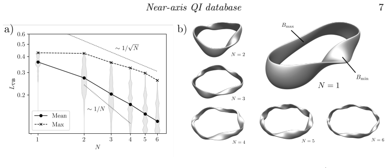
The paper claims that the near-axis expansion now enables a systematic, exhaustive mapping of quasi-isodynamic stellarator design space. Its construction parameterizes each configuration by eight scalars (axis curvature and torsion, on-axis field shape, flux-surface elongation), yielding a database of over 800,000 vacuum, approximately QI fields. Statistical analysis yields heuristics: the magnetic gradient scale is set mainly by torsion at the field minimum; MHD stability favors low integrated torsion and elongation stretching; maximum-J can exceed 80% at any field period; and effective ripple is the most restrictive measure. 'Good' configurations exist for N=1-5 but not N=6.
Load-bearing premise
The entire database assumes that a vacuum field's near-axis second-order expansion accurately represents a real stellarator equilibrium at finite aspect ratio, and in particular that first-order 'buffer' deviations from omnigeneity can be ignored when computing the effective ripple; if these approximations fail, the rankings and heuristics could change.
Editorial extensions
If this is right
- If the database is accurate, it provides thousands of baseline QI configurations that can serve as initial conditions for full-scale stellarator optimization, reducing the sensitivity of QI optimization to initial guesses.
- The heuristics indicate that lower field period numbers are systematically better for coil compatibility, MHD-stability shaping, and low neoclassical transport, while higher N improves beta resilience and zonal-flow support—quantifying the trade-off behind the choice of intermediate N in reactor designs.
- The figure-8-like configurations at N=2 stand out as the most compact stable configurations in the database, with aspect ratios around 2.3, offering a promising starting point for ultra-compact QI designs.
- Maximum-J behaviour can be achieved approximately at all field period numbers in a vacuum, with f_J exceeding 80% for the best cases, suggesting that turbulence-suppressing configurations need not be limited to low N.
- The effective ripple is the most restrictive 'goodness' criterion; no N=6 configurations satisfy all three thresholds, implying that transport-optimized high-N configurations require more flexible shaping than the current parameterization allows.
Reading between the lines
- If the database's near-axis heuristics survive global reconstruction, they imply a design principle not explicitly stated in the paper: the torsion at the field minimum, rather than average torsion, is the master parameter for coil-plasma distance. This could be used as a fast analytic proxy for coil complexity in future stellarator codes.
- A natural extension is to use the database to train a surrogate model that predicts epsilon_eff from the eight input scalars, enabling inverse design by gradient-based optimization directly in near-axis parameter space.
- The observed clustering into 'flat' and 'crown' families suggests distinct local minima in the design landscape; a testable hypothesis is whether these families are topologically distinct in terms of axis self-linking number or writhe, which might explain why optimization tends to converge to one family or the other.
- Because the database is limited to half-helicity, flattening class (2,3), and second order near-axis, the absence of 'good' N=6 configurations is not a fundamental bound; extending the parameterization (e.g., more Fourier harmonics in curvature/torsion or a different helicity) could plausibly produce good high-N configurations, and the database's structure can guide where to search.
Signed reviews
Editorial analysis
A structured set of objections, weighed in public.
Referee Report
Summary. The manuscript constructs a database of more than 800,000 near-axis quasi-isodynamic (QI) stellarator vacuum configurations, built from the authors' previously developed second-order near-axis construction with a restricted set of input parameters (axis torsion/curvature coefficients, elongation coefficients, mirror ratio, well-width parameter, and field period number). Each configuration is evaluated with near-axis measures: magnetic gradient scale L_∇B, critical aspect ratio A_mhd^c for a marginal vacuum well, maximum-J fraction f_J, effective ripple ε_eff, Shafranov shift sensitivity, and finite-orbit-width measures. The authors apply statistical tools (correlation, FSFS, PFI/cSAGE, clustering) to identify design heuristics, e.g. that low N favours coil compatibility and low ripple, high N favours high rotational transform and low Shafranov shift, and that maximum-J can be achieved at all N. The database is publicly released.
Significance. If the reported construction and diagnostics hold up, this is a valuable open resource: it maps a substantial, if deliberately restricted, part of near-axis QI design space and provides a large set of initial conditions for optimisation. The construction is internally careful — axis closure and first-order realness/periodicity are checked, and many measures are computed from parameter-free near-axis formulas rather than fitted to targets. The statistical analysis is thorough and reproducible in principle. The main weakness is the f_J computation, which omits a first-order non-omnigenous term that the manuscript itself says dominates near the axis; this could bias the maximum-J heuristics. The abstract's 'stable' also overstates the marginal W=0 vacuum-well nature of the representative configurations.
major comments (2)
- [Appendix D, §3.3, Eq. (D1) and Eq. (3.6)-(3.8), Table 6] The f_J computation uses only the O(r^0) omnigenous precession term ω_{α,vac} in Eq. (3.8), dropping the first-order non-QI term ω^{non-QI}_{α,-1}(λ) cos α / r shown in Eq. (D1). Appendix D itself states that this 1/r term 'dominate[s] precession sufficiently close to the magnetic axis, expecting f_J ≈ 0.5 there.' No estimate is given for the crossover radius r* = |ω^{non-QI}_{α,-1}|/|ω_{α,vac}|, nor is r* compared with the reference radius r_ref entering Eq. (3.6). Since Eq. (3.6) integrates with weight r dr from 0 to r_ref, the inner region contributes non-negligibly unless r* ≪ r_ref. If that condition is not met, the reported f_J maxima (Table 6: 0.86–0.91) are biased upward, and the conclusion in §3.3.2 and §4 that maximum-J is achievable at all N without excessive shaping may be an artifact. Please quantify r* for representative configurations across the database, or recompute f_J
- [Abstract, §1, §2, §3.2] The abstract and introduction describe the database as containing 'stable ... configurations', but the representative chosen for each first-order configuration is the marginal W=0 vacuum-well case (§2: 'marginal representative, W=0'; §3.2: 'marginally stable construction'). A vanishing vacuum well is a marginal condition, not a stable one, and A_mhd^c as defined in Eq. (3.3) is the aspect ratio at which the near-axis construction first breaks, not a demonstrated stability boundary. The 'stable' wording should be qualified as 'marginally stable (W=0)' in the abstract and wherever the database is summarised, to avoid overstating the physical content.
minor comments (4)
- [Appendix B and §3.1.2] The acronym SVR is used inconsistently: 'Statistical Vector Regression' in Appendix B.2, 'Statistical Virtual Regression' in the main text and later in Appendix B. Please use the standard 'Support Vector Regression' throughout.
- [Eq. (3.11)] The integral limits 'Z 1/Bmin over 1/Bmax' are difficult to read; the notation should be cleaned up (likely ∫_{1/Bmax}^{1/Bmin}).
- [Table 6] The superscript/subscript notation for maxima and minima (e.g. '0.43^0.12_0.27') is non-standard and hard to parse. Please define the notation explicitly in the caption or use a clearer format.
- [§3.4.1] The statement that the first-order buffer contribution ε_{eff}^{3/2,(0)} 'may be in practice ignored' would benefit from a quantitative justification — for example, citing the values in Table 6, which appear to be several orders of magnitude smaller than the ε_edge values used in the 'good' configuration criteria.
Circularity Check
No circular reduction: the database and heuristics are computed from independent near-axis formulas and descriptive statistics, not from fitting the target conclusions.
full rationale
The database is generated by scanning the stated input features and retaining configurations only if curve closure and first-order σ-equation periodicity/realness succeed. None of these filters use the physics diagnostics (L∇B, A_mhd^c, ϵeff, fJ) as targets, so the database is not constructed to force the reported trends. The diagnostics are evaluated from explicit near-axis formulas (Eqs. 3.1, 3.3, 3.10, 3.6-3.8) with stated assumptions; statistical conclusions (correlations, FSFS rankings, APM) are descriptive summaries of those computed values, not predictions obtained from fitted parameters that are then called independent. Self-citations to Plunk & Rodríguez (2026) and Rodriguez & Plunk (2025) transmit prior derivations with stated assumptions; they are not invoked as unverified uniqueness theorems and do not make the central claim definitional. The one caveat that could be mistaken for circularity is the use of ω_α≈ω_α,vac in Eq. (3.8): Appendix D explicitly notes the dropped 1/r buffer term dominates very close to the axis and would give fJ≈0.5 there, and no crossover radius is given. That is an internal correctness/validation risk, not a circular step, because the approximation is not fitted to or defined by the fJ values it is used to report. Overall the derivation chain is self-contained and the central claim (a public, code-generated database with stated near-axis assumptions) does not reduce to its inputs.
Assumptions & free parameters
free parameters (7)
- u =
2
- v =
3
- Nκ, Nτ =
2, 2
- helicity =
1/2
- W =
0
- B0 shape =
(1+λB, 1/4-2λB, -λB)
- scan ranges =
Table 4
assumptions (5)
- domain assumption Second-order near-axis expansion accurately describes finite-aspect-ratio quasi-isodynamic equilibria.
- ad hoc to paper First-order omnigeneity holds except in neglected buffer regions; buffer contributions to ε_eff are ignorable.
- ad hoc to paper The prescribed (κ, τ, ρ, B0) parameterization spans a representative subset of quasi-isodynamic stellarators.
- ad hoc to paper The marginal W=0 construction represents each first-order configuration's family for stability and shaping.
- standard math Vacuum magnetic well W governs MHD stability via Mercier's criterion in the low-beta limit.
Cite this review
Pith. "Pith review of Near-axis quasi-isodynamic database." pith.science (2026). https://pith.science/paper/R663LPU3
@misc{pith2026260108400,
  author       = {Pith},
  title        = {Pith review of: Near-axis quasi-isodynamic database},
  year         = {2026},
  howpublished = {\url{https://pith.science/paper/R663LPU3}},
  note         = {Machine review of arXiv:2601.08400}
}
read the original abstract
In this work, we investigate the landscape of quasi-isodynamic stellarators using the near-axis expansion of the magnetic field. Building on recent theoretical developments, we construct a database of more than 800,000 stable, approximately quasi-isodynamic vacuum magnetic configurations. These configurations span a range of field period numbers and other geometric control parameters, including the magnetic axis shape and plasma elongation. To evaluate each configuration, we use a broad set of measures, including effective ripple, sensitivity of the Shafranov shift to changes in plasma beta, the prevalence of maximum-J trapped particles, and the Rosenbluth-Hinton residual, among others. This enables an exhaustive, thorough and quantitative characterization of the database. Statistical analysis and modern machine learning techniques are then employed to find correlations, and identify key descriptors and heuristics to help understand tendencies that govern the behaviour of numerical optimization. The database provides baseline configurations for further studies, and to serve as tailored initial conditions for optimization. With this work we initiate a long term program to complete a systematic exploration of quasi-isodynamic stellarator design space.
Figures


Figures from the paper (23 more)


Forward citations
Cited by 2 Pith papers
-
Exploring the link between coil non-planarity and magnetic surface geometry across a dataset of QI stellarators
Statistical study of QI stellarator designs shows principal-direction rotation rate of the plasma boundary best predicts coil non-planarity, with surface features yielding Random Forest R²=0.882.
-
Equilibrium of a simplified coil quasi-axisymmetric stellarator: Free boundary approach
Optimized quasi-axisymmetric stellarator equilibria using a four-coil setup achieve reasonably good neoclassical transport for both vacuum and finite-pressure cases.
Reference graph
Works this paper leans on
-
[1]
CRC press
Animov, Yu2001Differential geometry and topology of curves. CRC press. Beidler, CD, Harmeyer, E, Herrnegger, F, Igitkhanov, Yu, Kendl, A, Kisslinger, J, Kolesnichenko, Ya I, Lutsenko, VV, Nührenberg, C, Sidorenko, I & others 2001 The helias reactor hsr4/18.Nuclear Fusion41(12),
2001
-
[3]
omnigenity near the magnetic axis.Journal of Plasma Physics 85(6), 905850602. Plunk, G. G. & Rodríguez, E.2026 A geometric approach to constructing quasi-isodynamic fields.Journal of Plasma Physics, in press, arXiv: 2508.12820. Pohl, William F1968 The self-linking number of a closed space curve.Journal of Mathematics and Mechanics17(10), 975–985. Proll, J...
arXiv 2026
-
[5]
Spitzer Jr, Lyman1958 The stellarator concept.The Physics of Fluids1(4), 253–264
New York - London: Consultants Bureau. Spitzer Jr, Lyman1958 The stellarator concept.The Physics of Fluids1(4), 253–264. Tenenbaum, Joshua B, Sil v a, Vin de & Langford, John C2000 A global geometric framework for nonlinear dimensionality reduction.science290(5500), 2319–2323. W armer, Felix, Alguacil, J, Biek, D, Bogaarts, T, Bongiovì, G, Bykov, V, Catal...
2025
-
[117]
Nührenberg, Jürgen2010 Development of quasi-isodynamic stellarators.Plasma Physics and Controlled Fusion52(12), 124003. 50E. Rodriguez, G. G. Plunk Oberti, Chiara & Ricca, Renzo L2016 On torus knots and unknots.Journal of Knot Theory and Its Ramifications25(06), 1650036. Panici, Dario, Rodriguez, Eduardo, Conlin, Rory, Dudt, Daniel & Kolemen, Egemen2025 E...
arXiv 2011
-
[213]
I., Shafranov, V
Mikhailov, M. I., Shafranov, V. D., Subbotin, A. A., Isaev, M. Y., Nührenberg, J., Zille, R. & Cooper, W. A.200242(11), L23–L26. Moff att, Henry Keith & Ricca, Renzo L1992 Helicity and the călugăreanu invariant. Proceedings of the Royal Society of London. Series A: Mathematical and Physical Sciences 439(1906), 411–429. Molnar, Christoph2020Interpretable m...
1906
-
[724]
Rosenbluth, M. N.1968 Low-frequency limit of interchange instability.The Physics of Fluids 11(4), 869–872, arXiv: https://aip.scitation.org/doi/pdf/10.1063/1.1692009. Sánchez, E., Velasco, J. L., Cal vo, I. & Mulas, S.2023 A quasi-isodynamic configuration with good confinement of fast ions at low plasmaβ.Nuclear Fusion63(6), 066037. Schölkopf, Bernhard & ...
-
[1759]
Bernardin, M. P., Moses, R. W. & Tataronis, J. A.1986 Isodynamical (omnigenous) equilibriuminsymmetricallyconfinedplasmaconfigurations.The Physics of Fluids29(8), 2605–2611. Blank, HJ de2004 Guiding center motion.Fusion science and technology45(2T), 47–54. 46E. Rodriguez, G. G. Plunk Figure 24:Feature dependence statistical summary forfJ. Figure 25:Featur...
arXiv 1986
-
[2830]
Pfefferlé, Da vid, Gunderson, Lee, Hudson, Stuart R & Noakes, Lyle2018 Non- planar elasticae as optimal curves for the magnetic axis of stellarators.Physics of Plasmas 25(9). Plunk, GG, Drevlak, M, Rodriguez, E, Babin, R, Goodman, A & Hindenlang, F 2024 Back to the figure-8 stellarator.arXiv preprint arXiv:2411.16411. Plunk, G. G., Landreman, M. & Helande...
arXiv 2024
Reviewed August 3, 2026 · model on record in the stance chip above.
Discussion (0). Continue with ORCID to comment.