Cauchy's Surface Area Formula in the Funk Geometry
Pith reviewed 2026-05-16 11:59 UTC · model grok-4.3
The pith
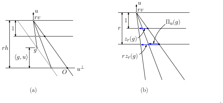
The Holmes-Thompson surface area in Funk geometry equals the average area of central projections onto the boundary of the inducing convex body.
A machine-rendered reading of the paper's core claim, the machinery that carries it, and where it could break.
Core claim
We establish an analog of Cauchy's formula for the Funk geometry induced by a convex body K in R^d, for the Holmes-Thompson surface area. The formula is based on central projections to boundary points of K. When K is a convex polytope, the formula reduces to a weighted sum of contributions associated with the vertices of K. As a consequence, we derive a generalization of Crofton's formula for surface areas in the Funk geometry.
What carries the argument
Central projections onto the boundary points of the convex body K, which replace the role of orthogonal projections in the Euclidean Cauchy formula.
If this is right
- When K is a convex polytope, the surface area formula reduces to a weighted sum over its vertices.
- The analysis yields a generalization of Crofton's formula in the Funk geometry.
- Euclidean, Minkowski, Hilbert, and hyperbolic surface area formulas arise as special cases of the Funk setting.
Where Pith is reading between the lines
- This approach could extend surface area computations to other Finsler geometries beyond Funk.
- Computational geometry algorithms for approximation might be adapted using this projection-based view.
- Verification on low-dimensional polytopes like simplices would provide immediate checks.
Load-bearing premise
That the Holmes-Thompson surface area is the right measure to use for the Funk geometry and that central projections play the same role as orthogonal projections do in Euclidean space.
What would settle it
Compute the Holmes-Thompson surface area of a specific convex body in a simple Funk geometry, such as a triangle in 2D, and check if it matches the average of its central projections onto the boundary; any mismatch would disprove the formula.
Figures





read the original abstract
Cauchy's surface area formula expresses the surface area of a convex body as the average area of its orthogonal projections over all directions. While this tool is fundamental in Euclidean geometry, with applications ranging from geometric tomography to approximation theory, extensions to non-Euclidean settings remain less explored. In this paper, we establish an analog of Cauchy's formula for the Funk geometry induced by a convex body $K$ in $\mathbb{R}^d$, for the Holmes--Thompson surface area. The formula is based on central projections to boundary points of $K$. We show that when $K$ is a convex polytope, the formula reduces to a weighted sum of contributions associated with the vertices of $K$. Finally, as a consequence of our analysis, we derive a generalization of Crofton's formula for surface areas in the Funk geometry. By viewing Euclidean, Minkowski, Hilbert, and hyperbolic geometries as limiting or special cases of the Funk setting, our results provide a unified framework for these classical surface area formulas.
Editorial analysis
A structured set of objections, weighed in public.
Referee Report
Summary. The manuscript establishes an analog of Cauchy's surface area formula in the Funk geometry induced by a convex body K in R^d, expressed in terms of the Holmes-Thompson surface area and using central projections onto boundary points of K. For polytopes the formula reduces to a vertex-weighted sum; a Crofton-type generalization for surface areas is also derived. The work frames Euclidean, Minkowski, Hilbert, and hyperbolic geometries as limiting or special cases of the Funk setting.
Significance. If the central derivation holds, the result supplies a unified framework for classical surface-area formulas across several geometries, which would be of interest to researchers in convex geometry, Finsler geometry, and geometric tomography. The explicit polytope reduction and the Crofton generalization constitute concrete, checkable contributions.
major comments (2)
- [§3] §3, Theorem 3.1: the statement that the Holmes-Thompson area equals the average of central projections requires an explicit verification that the Funk metric's unit ball induces the correct normalization; without the intermediate integral identity (presumably Eq. (8)), it is unclear whether the constant factor matches the Euclidean limit.
- [§4] §4, Proposition 4.2: the reduction to a vertex-weighted sum for polytopes is asserted to follow from the general formula, but the weights are defined via the support function of K; a direct computation for the simplex in R^3 should be added to confirm the weights are independent of the choice of origin inside K.
minor comments (2)
- The notation for the central projection map (p. 7) uses the same symbol as the boundary point; a distinct symbol would improve readability.
- Reference list omits the 2018 paper by Alvarez and Berck on Holmes-Thompson volume in Finsler spaces; adding it would strengthen the background section.
Simulated Author's Rebuttal
We thank the referee for the careful reading and constructive comments on our manuscript. We address each major comment below and will revise the manuscript to incorporate the suggested clarifications.
read point-by-point responses
-
Referee: §3, Theorem 3.1: the statement that the Holmes-Thompson area equals the average of central projections requires an explicit verification that the Funk metric's unit ball induces the correct normalization; without the intermediate integral identity (presumably Eq. (8)), it is unclear whether the constant factor matches the Euclidean limit.
Authors: We agree that an explicit verification of the normalization is necessary for clarity. In the revised version we will insert the intermediate integral identity (now explicitly labeled as Equation (8)) and include a short computation confirming that the constant factor recovers the classical Euclidean value in the appropriate limit. revision: yes
-
Referee: §4, Proposition 4.2: the reduction to a vertex-weighted sum for polytopes is asserted to follow from the general formula, but the weights are defined via the support function of K; a direct computation for the simplex in R^3 should be added to confirm the weights are independent of the choice of origin inside K.
Authors: We accept the suggestion. The revised manuscript will contain an explicit direct computation for the standard 3-simplex in R^3, verifying that the vertex weights (expressed through the support function of K) remain unchanged under any choice of origin in the interior of K. revision: yes
Circularity Check
No significant circularity detected in derivation
full rationale
The paper derives an analog of Cauchy's surface area formula in Funk geometry induced by convex body K, using Holmes-Thompson surface area and central projections onto bd(K). The abstract describes the result as holding for general convex K, reducing to vertex-weighted sums for polytopes, and yielding a Crofton generalization as a consequence. No load-bearing step reduces by the paper's own equations to a fitted input, self-definition, or prior self-citation chain; the unification with Euclidean/Minkowski/Hilbert/hyperbolic cases is presented as a limiting consequence rather than an imported ansatz or uniqueness theorem. The derivation chain is self-contained against the stated geometric assumptions and does not exhibit any of the enumerated circularity patterns.
Axiom & Free-Parameter Ledger
Lean theorems connected to this paper
-
IndisputableMonolith/Cost/FunctionalEquation.leanwashburn_uniqueness_aczel unclear?
unclearRelation between the paper passage and the cited Recognition theorem.
areaF_K(G) = 1/ω_{d-1} ∫_{S^{d-1}} λ_{d-1}(S_K(G,u)) dσ(u) ... based on central projections to boundary points of K
-
IndisputableMonolith/Foundation/AlexanderDuality.leanalexander_duality_circle_linking unclear?
unclearRelation between the paper passage and the cited Recognition theorem.
Lemma 2.1 (Projection-Section Duality) ... (K∩E)^∘_E = K^∘ |_E
What do these tags mean?
- matches
- The paper's claim is directly supported by a theorem in the formal canon.
- supports
- The theorem supports part of the paper's argument, but the paper may add assumptions or extra steps.
- extends
- The paper goes beyond the formal theorem; the theorem is a base layer rather than the whole result.
- uses
- The paper appears to rely on the theorem as machinery.
- contradicts
- The paper's claim conflicts with a theorem or certificate in the canon.
- unclear
- Pith found a possible connection, but the passage is too broad, indirect, or ambiguous to say the theorem truly supports the claim.
Forward citations
Cited by 1 Pith paper
-
On the Duality of Coverings in Hilbert Geometry
Hilbert-geometry covering numbers satisfy polarity duality: N^H_K(G, α) is bounded above and below by c^{±d} times N^H_{G°}(K°, α) for an absolute constant c.
Reference graph
Works this paper leans on
-
[1]
C. Aaron, A. Cholaquidis, and R. Fraiman. Estimation of surface area.Electronic Journal of Statistics, 16(2):3751–3788, 2022.doi:10.1214/22-EJS2031
-
[2]
A Geometric Heuristic for Rectilinear Crossing Minimization
A. Abdelkader and D. M. Mount. Convex approximation and the Hilbert geometry. InProc. SIAM Symp. Simplicity in Algorithms (SOSA24), pages 286–298, 2024.doi:10.1137/1. 9781611977936.26
work page doi:10.1137/1 2024
-
[3]
P. K. Agarwal, S. Har-Peled, and K. R. Varadarajan. Approximating extent measures of points.J. Assoc. Comput. Mach., 51:606–635, 2004.doi:10.1145/1008731.1008736
-
[4]
R. Alexander. Planes for which the lines are the shortest paths between points.Ill. J. Math., 22:177–190, 1978.doi:10.1215/ijm/1256048729
-
[5]
R. Alexander, I. D. Berg, and R. L. Foote. Integral-geometric formulas for perimeter in S2,H 2, and Hilbert planes.Rocky Mountain J. Mathematics, 35(6):1825–1859, 2005. URL: http://www.jstor.org/stable/44238783
-
[6]
J. C. ´Alvarez Paiva and E. Fernandes. Crofton formulas in projective Finsler spaces.Electron. Res. Announc. Amer. Math. Soc., 4:91–100, 1998. URL:http://eudml.org/doc/224916
work page 1998
-
[7]
R. Arya, S. Arya, G. D. da Fonseca, and D. M. Mount. Optimal bound on the combinatorial complexity of approximating polytopes.ACM Trans. Algorithms, 18:1–29, 2022.doi:10. 1145/3559106
work page 2022
-
[8]
S. Arya, G. D. da Fonseca, and D. M. Mount. Economical convex coverings and applications. SIAM J. Comput., 53(4):1002–1038, 2024.doi:10.1137/23M1568351
-
[9]
A. Baddeley and E. B. V. Jensen.Stereology for Statisticians. CRC Press, 2005.doi: 10.1201/9780203496817
-
[10]
Barvinok.A Course in Convexity, volume 54 ofGraduate Studies in Mathematics
A. Barvinok.A Course in Convexity, volume 54 ofGraduate Studies in Mathematics. American Mathematical Society, 2002. URL:https://bookstore.ams.org/gsm-54/
work page 2002
-
[11]
J.-D. Boissonnat, F. Nielsen, and R. Nock. Bregman Voronoi diagrams.Discrete Comput. Geom., 44:281–307, 2010.doi:10.1007/s00454-010-9256-1
-
[12]
J. W. Cannon, W. J. Floyd, R. Kenyon, and W. R. Parry. Hyperbolic geometry. In S. Levy, editor,Flavors of Geometry, volume 31 ofMSRI Publications, pages 59–115. Cambridge Uni- versity Press, 1997
work page 1997
-
[13]
K. L. Clarkson. Building triangulations usingε-nets. InProc. 38th Annu. ACM Sympos. Theory Comput., pages 326–335, 2006.doi:10.1145/1132516.1132564
-
[14]
M. P. do Carmo.Differential Geometry of Curves and Surfaces. Prentice Hall, 1976
work page 1976
-
[15]
D. Faifman. A Funk perspective on billiards, projective geometry and Mahler volume.J. Differential Geom., 127:161–212, 2024.doi:10.4310/jdg/1717356157
-
[16]
D. Faifman, C. Vernicos, and C. Walsh. Volume growth of Funk geometry and the flags of polytopes.Geometry & Topology, 29(7):3773–3811, 2025.doi:10.2140/gt.2025.29.3773. 23
-
[17]
R. J. Gardner.Geometric Tomography. Cambridge University Press, 2nd edition, 2006.doi: 10.1017/CBO9781107341029
-
[18]
R. D. Holmes and A. C. Thompson.n-dimensional area and content in Minkowski spaces. Pacific J. Math., 85:77–110, 1979.doi:10.2140/pjm.1979.85.77
-
[19]
M. Ito, Y. Seo, T. Yamazaki, and M. Yanagida. Geometric properties of positive definite matrices cone with respect to the Thompson metric.Linear Algebra Appl., 435:2054–2064, 2011.doi:10.1016/j.laa.2011.03.063
-
[20]
D. Krioukov, F. Papadopoulos, M. Kitsak, A. Vahdat, and M. Bogu˜ n´ a. Hyperbolic geometry of complex networks.Phys. Rev. E, 82, 2010.doi:10.1103/PhysRevE.82.036106
-
[21]
A. A. Kurzhanskiy and P. Varaiya. Ellipsoidal toolbox. Technical Report UCB/EECS-2006- 46, EECS Department, University of California, Berkeley, 2006. URL:https://www2.eecs. berkeley.edu/Pubs/TechRpts/2006/EECS-2006-46.html
work page 2006
-
[22]
X. Li, W. Wang, R. R. Martin, and A. Bowyer. Using low-discrepancy sequences and the crofton formula to compute surface areas of geometric models.Computer-Aided Design, 35(9):771–782, 2003.doi:10.1016/S0010-4485(02)00100-8
-
[23]
W. Lin, V. Duruisseaux, M. Leok, F. Nielsen, M. E. Khan, and M. Schmidt. Simplifying momentum-based positive-definite submanifold optimization with applications to deep learn- ing. InProc. 40th Internat. Conf. Mach. Learn., 2023. URL:https://arxiv.org/abs/2302. 09738
work page 2023
-
[24]
Y.-S. Liu, J. Yi, H. Zhang, G.-Q. Zheng, and J.-C. Paul. Surface area estimation of digitized 3d objects using quasi-monte carlo methods.Pattern Recognition, 43:3900–3909, 2010.doi: 10.1016/j.patcog.2010.06.002
-
[25]
F. Nielsen and K. Sun. Clustering in Hilbert’s projective geometry: The case studies of the probability simplex and the elliptope of correlation matrices. InGeometric Structures of Information, Signals and communication technology, pages 297–331. Springer International Publishing, 2019.doi:10.1007/978-3-030-02520-5_11
-
[26]
A. Papadopoulos and M. Troyanov. Harmonic symmetrization of convex sets and of Finsler structures, with applications to Hilbert geometry.Expo. Math., 27:109–124, 2009.doi:10. 1016/j.exmath.2008.10.001
work page 2009
-
[27]
A. Papadopoulos and M. Troyanov.Handbook of Hilbert Geometry. EMS Press, 2014.doi: 10.4171/147
work page doi:10.4171/147 2014
-
[28]
R. T. Rockafellar.Convex Analysis. Princeton University Press, Princeton, NJ, 1997.doi: 10.1515/9781400873173
-
[29]
Rudin.Real and Complex Analysis
W. Rudin.Real and Complex Analysis. McGraw Hill, 3rd edition, 1987
work page 1987
-
[30]
R. Schneider. Crofton formulas in hypermetric projective Finsler spaces.Archiv der Mathe- matik, 77:85–97, 2001.doi:10.1007/PL00000469
- [31]
-
[32]
R. Schneider. Crofton measures in projective Finsler spaces. In E. L. Grinberg, S. Li, G. Zhang, and J. Zhou, editors,Integral Geometry and Convexity, pages 67–98. World Scientific, 2006. doi:10.1142/9789812774644_0006
-
[33]
R. Schneider.Convex Bodies: The Brunn-Minkowski Theory, volume 151 ofEncyclopedia of Mathematics and its Applications. Cambridge Univ. Press, 2nd edition, 2014.doi:10.1017/ CBO9781139003858
work page 2014
-
[34]
A. C. Thompson.Minkowski Geometry, volume 63 ofEncyclopedia of mathematics and its applications. Cambridge University Press, 1996.doi:10.1017/CBO9781107325845
-
[35]
M. Troyanov. Funk and Hilbert geometries from the Finslerian viewpoint. InHandbook of Hilbert geometry, pages 69–110. European Mathematical Society Publishing House, 2014.doi: 10.4171/147-1/3
-
[36]
Springer-Verlag, New York, 1995, pp
G¨ unter M. Ziegler.Lectures on Polytopes, volume 152 ofGraduate Texts in Mathematics. Springer-Verlag, New York, 1995.doi:10.1007/978-1-4613-8431-1. A Justification of the Cone Volume Definition The definition of the Funk volume for cones (Eq. (4)) relies on an integration over the cone’s spherical cross-section. To justify this definition, we must show ...
discussion (0)
Sign in with ORCID, Apple, or X to comment. Anyone can read and Pith papers without signing in.