REVIEW 4 major objections 5 minor 176 references
Discovering Interpretable Algorithms by Decompiling Transformers to RASP
T0 review · 4 major / 5 minor · reviewed 2026-08-03 · deepseek-v4-flash
Pith's one-line read This paper claims that small transformers that length-generalize on algorithmic and formal-language tasks can be decompiled into short, human-readable RASP programs, and presents an automatic method that does so.
desk verdict Genuinely new decompilation pipeline that recovers compact RASP programs from trained small transformers; the central 'internally implement' claim rests on a 90% match-accuracy criterion, so treat extracted programs as fitted surrogates until exact or unique match is shown. read the letter →
The pith
A machine-rendered reading of the paper's core claim, the machinery that carries it, and where it could break.
The reading
What carries the argument
The central object is D-RASP (Decompiled RASP), a RASP dialect using softmax aggregation and one-hot token and position variables, designed so transformer computations can be faithfully represented. Theorem 3.2 shows that any GPT-2-style transformer satisfying the linear layer norm assumption can be exactly translated into a D-RASP program by tracking each path through the residual stream as a separate variable. Because the naive translation is exponentially large, the load-bearing mechanism is the causal-pruning step: trainable masks and optimal ablations remove causally irrelevant components, and a library of primitives replaces learned matrices and per-position maps with named operations
What would settle it
Take one of the decompiled programs and evaluate it on a deliberately constructed set of inputs where it disagrees with the original model, including lengths beyond the training range; if the model generalizes correctly on those inputs while the program fails, then the extracted program is not the algorithm driving the model's behavior.
Extended reading notes
Core claim
The central discovery is that the inverse of compiling RASP to transformers works: a trained transformer can be translated back into a readable program. Under the Linear Layer Norm Assumption, every GPT-2-style transformer has an exact D-RASP representation whose variables live in interpretable spaces such as token identities and positions, and causal pruning can reduce the exponentially large naive translation to a few lines that still match the original model on at least 90 percent of random inputs. On algorithmic and formal-language tasks, the method recovers compact programs that recapitulate known mechanisms—uniform aggregation computing a histogram for most-frequent, an off-by-one sele
Load-bearing premise
The load-bearing premise is that matching the model's predictions on at least 90 percent of random inputs—after assuming layer norms can be replaced by linear maps—is enough to conclude the extracted program is the algorithm the transformer internally implements.
Editorial extensions
If this is right
- If decompilability tracks length generalization, then successful length generalization in these settings is accompanied by an extractable symbolic algorithm, strengthening the RASP length-generalization conjecture.
- The extracted programs apply uniformly over input lengths, unlike circuits found by circuit discovery, so they can explain behavior on out-of-distribution lengths rather than only training templates.
- Because D-RASP program size is independent of hidden dimension, even overparameterized models can yield small interpretable programs.
- The recovered programs match mechanisms hypothesized in prior theory, providing independent confirmation of those hypotheses.
- The method offers a practical pipeline for future interpretability work: reparameterize faithfully, prune causally, then name operations with primitives.
Reading between the lines
- I would treat a successful decompilation as a strong hypothesis about the model's algorithm rather than a proof: the 90 percent match threshold means a program could disagree with the model on the remaining inputs, including the long sequences where generalization is actually being tested.
- If the correlation holds more broadly, decompilability itself could serve as a diagnostic: run the pipeline on a model and use whether a compact program emerges as a proxy for whether it will length-generalize.
- The same reparameterize-and-prune recipe might be adapted to larger language models by decompiling individual subtasks rather than the whole model, though the paper does not claim this.
- A natural testable extension is to compile the extracted programs back into transformers and check behavioral equivalence on adversarial inputs, which would sharpen the faithfulness question.
Editorial analysis
A structured set of objections, weighed in public.
Referee Report
Summary. The paper proposes a decompilation pipeline that translates small GPT-2-style transformers into programs in a new RASP dialect, D-RASP, and then prunes/simplifies these programs to obtain compact, human-readable algorithms. The authors prove (Theorem 3.2, under a linear layer-norm assumption) that a transformer can be exactly reparameterized as a D-RASP program, and they validate the simplification stage empirically by requiring the extracted program to match the original model's predictions on ≥90% of random i.i.d. inputs of length up to 150. On a suite of algorithmic and formal-language tasks, they report that length-generalizing models are usually decompilable while non-length-generalizing models are not, and they present several recovered programs that align with known algorithmic motifs such as histogram-based majority, induction-head copying, and bounded-depth Dyck recognition.
Significance. If the central claim holds, this is a valuable contribution to mechanistic interpretability: it would provide the first automated extraction of symbolic, length-generalizing programs from normally trained transformers, connecting the RASP length-generalization conjecture to actual trained models. The paper includes a detailed proof of exact reparameterization under LLNA, extensive appendices with per-task programs, and a public code link, all of which are strengths. The recovered programs for tasks like Unique Copy and Most Frequent are genuinely interpretable and match prior theoretical expectations. However, the significance is tempered by the fact that the main empirical claim rests on a 90% match-accuracy threshold rather than exact equivalence, and the experimental protocol selects the best length-generalizing model per task without repeated-seed error bars. These issues do not invalidate the method but do weaken the strong wording 'most direct evidence so far that Transformers internally implement simple RASP programs.'
major comments (4)
- [§3.2, FAQ 8] The central faithfulness criterion is behavioral match accuracy ≥90% on random i.i.d. inputs of length ≤150, explicitly chosen 'based on common sense.' This threshold does not establish that the extracted program is the algorithm the transformer internally implements: a program agreeing on 90% of inputs can differ on the remaining 10%, including precisely the structured or out-of-distribution inputs most relevant to length generalization. The exactness guarantee in Theorem 3.2 holds only before the simplification steps; every subsequent step (causal pruning, primitive replacement, matrix rounding) is validated by aggregated match accuracy with additional thresholds (0.92, 0.95×, 0.91× in Apps. G–H). The paper should either provide exact or near-exact equivalence checks on held-out and OOD length ranges, or substantially soften the claim that decompilation recovers the internal algorithm.
- [§4, Tables 1 and 2] The models analyzed are selected as the best length-generalizers from a hyperparameter sweep, with no repeated-seed variance or error bars. The claim that 'length-generalizing models can be decompiled and non-length-generalizing models cannot' is therefore not yet supported as a general empirical law. Moreover, Table 2 itself lists five length-generalizing formal-language models where LLNA does not hold (Tomita4, D3, (aaaa)*, (abab)*, {0,1,2}*02*), and D12 succeeds only after a post-hoc threshold adjustment. The paper acknowledges these exceptions but should analyze them more directly, e.g., by reporting whether these models are nevertheless decomposable into interpretable programs under a weaker notion of faithfulness.
- [§3.2, App. F–H] There is an element of circularity in the success criterion: the pipeline fits sparse coefficients, primitive replacements, and integer/rounded matrices to maximize match accuracy, and then declares success when match accuracy exceeds 90%. This means the extracted program is partly a fitted surrogate rather than an independently discovered cause. To break the circularity, the authors should validate a few extracted programs by testing their causal predictions on the original model—e.g., by intervening on the model's internal components in the way the program describes and showing that behavior changes accordingly—or by demonstrating that the program predicts model behavior on adversarial, structured inputs that were not used during pruning.
- [Theorem 3.2, Assumption 3.1] The exact reparameterization theorem relies critically on LLNA, yet LLNA is an empirical assumption that fails for a non-negligible subset of the paper's own length-generalizing models (Table 2). The paper states that the pipeline requires LLNA, but the abstract and introduction present the method as general ('a general method to extract such programs from trained Transformers'). The scope should be stated more precisely in the main text, and the authors should discuss whether the LLNA failure cases are a limitation of the method or evidence that those models use genuinely non-linear layer-norm computations.
minor comments (5)
- [Throughout] There are repeated typos and informal phrases: 'reparamaterization' (§3 header), 'strinfs' (App. J.3), 'preogram' (App. J.10). The paper would benefit from a careful proofreading pass.
- [§4, Table 2] The special cases marked with ×* are explained only in footnotes; a short paragraph in the main text explaining why D12 and D2 are still counted as successes would improve transparency.
- [App. F.1, Eq. 19] The sparsity regularizer R(θ̃) is described as 'the expected number of edges' but the exact form is not given; please provide the explicit expression for R.
- [App. H, Table 3] The primitive names such as 'op=(k==q-k)' are confusing: the subscript k appears both as a variable and as a constant offset. Please use distinct notation, e.g., 'k == q - c'.
- [§3.1, Theorem 3.2] The proof in Appendix B.3 is detailed, but the main-text description of the exponential blow-up and the multi-stage pruning used to avoid it would benefit from a small illustrative example in the main text, not only in the appendix.
Circularity Check
No significant circularity: the simplified programs are fitted to the model, but the empirical claim that simple programs are recoverable is not tautological and no load-bearing step reduces to a self-citation.
full rationale
The derivation has two independent parts. Theorem 3.2 (App. B.3) gives an explicit, exact translation from an LLNA-satisfying GPT-2 transformer to a D-RASP program, with a self-contained induction proof of equality of the input-output map; this is a construction, not a circular prediction. The second part is an empirical search over pruned programs validated by match accuracy. Because the simplification pipeline selects programs using the same match-accuracy criterion, the reported match accuracies are post-fit quantities, but the paper does not present them as held-out predictions. The phrase "we deem decompilation to be causally faithful when the match accuracy is ≥90%" (Sec. 3.2) and the statement that this threshold was "chosen based on common sense" (FAQ 8) show that the faithfulness criterion is a stated convention, not a conclusion derived from the model. One can question whether 90% behavioral match on i.i.d. inputs is enough to establish that the extracted program is the unique internal algorithm, and the paper itself acknowledges that Assumption 3.1 (LLNA) fails for some length-generalizing formal-language models (Table 2, App. E). But those are validity/calibration concerns, not circularity: nothing defines the target result into existence. The cited RASP length-generalization conjecture (Zhou et al. 2024; Huang et al. 2025) is used as motivation and context, not as a load-bearing proof step, and the LLNA motivation is external (Baroni et al. 2025). Self-citations are present but non-load-bearing, so no circular step is exhibited.
Assumptions & free parameters
free parameters (4)
- Layer-normalization linearization constants gamma' =
per-layer, not reported numerically
- Match-accuracy threshold =
0.9
- Sparsity coefficients lambda =
swept; values not fixed
- Primitive-matching thresholds and primitive hyperparameters =
0.92, 0.9, 0.95x, 0.91x; n in {2,3,5}, tau in {0.7,...,0.95}
assumptions (4)
- domain assumption Linear Layer Norm Assumption: each LayerNorm can be replaced by a linear map (x - mean)gamma' + beta with negligible change (Assumption 3.1).
- domain assumption GPT-2-style architecture with absolute positional embeddings, softmax attention, one-layer MLPs, and causal masking.
- domain assumption D-RASP/C-RASP equivalence assumes p-bit rounded semantics and rational tensor entries (Theorem 2.1).
- domain assumption The RASP length-generalization conjecture from prior work is accepted as background for interpreting recovered programs.
invented entities (1)
-
D-RASP (Decompiled RASP)
independent evidence
Cite this review
Pith. "Pith review of Discovering Interpretable Algorithms by Decompiling Transformers to RASP." pith.science (2026). https://pith.science/paper/3AFBIADC
@misc{pith2026260208857,
  author       = {Pith},
  title        = {Pith review of: Discovering Interpretable Algorithms by Decompiling Transformers to RASP},
  year         = {2026},
  howpublished = {\url{https://pith.science/paper/3AFBIADC}},
  note         = {Machine review of arXiv:2602.08857}
}
read the original abstract
Recent work has shown that the computations of Transformers can be simulated in the RASP family of programming languages. These findings have enabled improved understanding of the expressive capacity and generalization abilities of Transformers. In particular, Transformers have been suggested to length-generalize exactly on problems that have simple RASP programs. However, it remains open whether trained models actually implement simple interpretable programs. In this paper, we present a general method to extract such programs from trained Transformers. The idea is to faithfully re-parameterize a Transformer as a RASP program and then apply causal interventions to discover a small sufficient sub-program. In experiments on small Transformers trained on algorithmic and formal language tasks, we show that our method often recovers simple and interpretable RASP programs from length-generalizing transformers. Our results provide the most direct evidence so far that Transformers internally implement simple RASP programs.
Figures


Figures from the paper (88 more)






Reference graph
Works this paper leans on
-
[1]
For eachx∈start,⟨x,⟨⟩⟩ ∈ V
-
[2]
For anyl∈[L], h∈[H], wheneverlayer(⟨x, p⟩)< land⟨x, p⟩ ∈ V, then⟨x,⟨(l, h)⟩ ⊕p⟩ ∈ V. where 3.layer(⟨tok, p⟩) :=layer(p) 4.layer(⟨pos, p⟩) :=layer(p) 5.layer(⟨mlp k, p⟩) := max(k, layer(p)) 14 Interpretable Algorithms by Decompiling Transformers In particular, eachv∈ Vis a tuple consisting ofx∈startand a pathp. For each⟨i, p⟩ ∈ V, our D-RASP program will h...
-
[5]
Haklay, T., Orgad, H., Bau, D., Mueller, A., and Belinkov, Y
URL https://openreview.net/forum? id=Pe9WxkN8Ff. Haklay, T., Orgad, H., Bau, D., Mueller, A., and Belinkov, Y . Position-aware automatic circuit discovery. In Che, W., Nabende, J., Shutova, E., and Pilehvar, M. T. (eds.),Pro- ceedings of the 63rd Annual Meeting of the Association for Computational Linguistics (Volume 1: Long Papers), pp. 2792–2817, Vienna...
2025
-
[6]
URL https: //aclanthology.org/2025.acl-long.141/
doi: 10.18653/v1/2025.acl-long.141. URL https: //aclanthology.org/2025.acl-long.141/. Hanna, M., Liu, O., and Variengien, A. How does gpt-2 compute greater-than?: Interpreting mathematical abili- ties in a pre-trained language model.Advances in Neu- ral Information Processing Systems, 36:76033–76060, 9 Interpretable Algorithms by Decompiling Transformers
-
[7]
Huang, X., Yang, A., Bhattamishra, S., Sarrof, Y ., Krebs, A., Zhou, H., Nakkiran, P., and Hahn, M
URL https://openreview.net/forum? id=p4PckNQR8k. Huang, X., Yang, A., Bhattamishra, S., Sarrof, Y ., Krebs, A., Zhou, H., Nakkiran, P., and Hahn, M. A formal framework for understanding length generalization in transformers. InThe Thirteenth International Conference on Learning Representations, 2025. URL https:// openreview.net/forum?id=U49N5V51rU. Izzo, ...
arXiv 2025
-
[9]
Langosco, L., Baker, W., Alex, N., Bradley, H., Quarel, D., and Krueger, D
URL https://openreview.net/forum? id=W8K8slZ73R. Langosco, L., Baker, W., Alex, N., Bradley, H., Quarel, D., and Krueger, D. Towards meta-models for automated interpretability, 2024. URL https://openreview. net/forum?id=1zDOkoZAtl. Li, J. and Cotterell, R. Characterizing the expressivity of fixed-precision transformer language models. In The Thirty-ninth ...
2024
-
[10]
Liu, B., Ash, J., Goel, S., Krishnamurthy, A., and Zhang, C
URL https://openreview.net/forum? id=tbbId8u7nP. Liu, B., Ash, J., Goel, S., Krishnamurthy, A., and Zhang, C. Exposing attention glitches with flip-flop language modeling.Advances in Neural Information Process- ing Systems, 36:25549–25583, 2023. URL https: //openreview.net/forum?id=VzmpXQAn6E. Merrill, W. and Sabharwal, A. A logic for express- ing log-pre...
2023
-
[11]
URL https://openreview.net/forum? id=uR8TtWCIsr. nostalgebraist. interpreting gpt: the logit lens.LESS- WRONG, 2020. https://www.lesswrong. com/posts/AcKRB8wDpdaN6v6ru/ interpreting-gpt-the-logit-lens. Olsson, C., Elhage, N., Nanda, N., Joseph, N., Das- Sarma, N., Henighan, T., Mann, B., Askell, A., Bai, Y ., Chen, A., Conerly, T., Drain, D., Ganguli, D.,...
Show all 176 references
-
[12]
tacl-1.9/
URL https://aclanthology.org/2025. tacl-1.9/. Thurnherr, H. and Riesen, K.Neural Decompiling of Tracr Transformers, pp. 25–36. Springer Nature Switzer- land, 2024. ISBN 9783031716027. doi: 10.1007/ 978-3-031-71602-7 3. URL http://dx.doi.org/ 10.1007/978-3-031-71602-7_3. Wang, ...
2025 doi
-
[13]
Weiss, G., Goldberg, Y ., and Yahav, E
URL https://openreview.net/forum? id=NpsVSN6o4ul. Weiss, G., Goldberg, Y ., and Yahav, E. Thinking like transformers. InInternational Conference on Machine Learning, pp. 11080–11090. PMLR, 2021. URL http://proceedings.mlr.press/v139/ weiss21a.html. 10 Interpretable Algorithms ...
2021
-
[14]
URL https://openreview.net/forum? id=OitmaxSAUu. Yang, A. and Chiang, D. Counting like transformers: Compiling temporal counting logic into softmax trans- formers. InFirst Conference on Language Modeling,
-
[15]
Yang, A., Chiang, D., and Angluin, D
URL https://openreview.net/forum? id=FmhPg4UJ9K. Yang, A., Chiang, D., and Angluin, D. Masked hard- attention transformers recognize exactly the star-free languages.Advances in Neural Information Process- ing Systems, 37:10202–10235, 2024. URL https: //openreview.net/forum?id=...
2024
-
[16]
logits5 = project(inp=a1, op= g )
-
[17]
How does D-RASP compare to Transformer Programs (Friedman et al., 2023; Lai-Dang et al., 2025) and the Discrete Transformer (Zhang et al., 2026)? On a technical level, there are some similarities; in particular, our definition of separate variables for each path through the re...
2023
-
[18]
logits7 = project(inp=is_01_balance_a3, op= i )
-
[19]
logits8 = project(inp=pos, op= m )
-
[25]
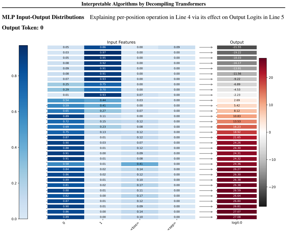
a2 = aggregate(s=s1+s2+s3+s4, v=pos) Defining elementwise operationsWe set Line performing per-position operation v⟨mlpl,⟨⟩⟩ =element wise op(vs(i) :s∈ V − {vmlp,l}, layer(s)≤l,func=f) wherefoutputs the output vector of the original MLPf M LP,lof thel-th layer: f v(s,p)(i) : (...
-
[26]
m = element_wise_op(token+pos+a1+a2) Treating Unembedding MatricesWe define the unembedding projections as R⟨i,p⟩ =U Y ⟨l′,h′⟩∈p Vh′,l′ T(i)(13) for each⟨i, p⟩withlayer(p)≤L, and set 16 Interpretable Algorithms by Decompiling Transformers Line performing per-position o...
-
[32]
Line defining a selector
prediction = softmax(logits1+logits2+logits3+logits4+logits5) B.4. Proof of Theorem 3.2 Theorem B.2(Restated from Theorem 3.2).Consider a GPT-2-style transformer satisfying LLNA. There is a D-RASP program defining the same input-output map; it can be explicitly obtained from t...
-
[37]
a1 = aggregate(s=s1+s2+s3+s4, v=token)
-
[45]
prediction = softmax(logits1+logits2+logits3+logits4+logits5) After pruning:
-
[46]
s1 = select(q=token, k=token)
-
[47]
s2 = select(q=token, k=pos)
-
[48]
s3 = select(q=pos, k=token)
-
[49]
s4 = select(q=pos, k=pos)
-
[50]
a1 = aggregate(s=s1 +s2+s3+s4, v=token)
-
[51]
a2 = aggregate(s=s1+s2+s3+s4, v=pos)
-
[52]
m = elementwise_op(token+pos+a1+a2)
-
[53]
logits1 = project(token)
-
[54]
logits2 = project(pos)
-
[55]
logits3 = project(a1)
-
[56]
logits4 = project(a2)
-
[57]
logits5 = project(m)
-
[58]
define the same functions
prediction = softmax( logits1+logits2+logits3+logits4+logits5) Figure 9.See text. B.6. Size of D-RASP Translation The size of the D-RASP translation given by Theorem 3.2 is given by: def determine_total_line(num_layer, num_head, split_mlps): num_v = 2 num_line = 0 for i in ran...
2025
-
[59]
We can see that very different architectures can all be decompilable (e.g., two green lines in Figure 10(a) correspond to 4 layer vs
For each task, we show 2-3 models different architectures. We can see that very different architectures can all be decompilable (e.g., two green lines in Figure 10(a) correspond to 4 layer vs. 2 layer models), while similar architectures can exhibit different decompilability (...
1900
-
[60]
Columns of v is the result of per-column operation of x, i.e., v(i) only depends on x(i)
Collect output activations v∈R d×N (see method in Appendix F.2) of the target MLP (which is also activation variables before finding a primitive), and activation variables x∈R d(x)×N (see method in Appendix G.1) of its inputs. Columns of v is the result of per-column operation...
-
[61]
Test primitives. For each primitivef j in the single input primitive list, do the following: (a) Obtain the transformed activation variables w∈R d(w)×N by applying fj to x (i.e., w(i) = element wise op(x(i),func=f s)).d(w)depends on the output dimension off j. (b) Obtain a lin...
-
[62]
Importantly, to simplify the generated program, we favor replacing MLP with linear operation, i.e., fno−op
Select the best primitive. Importantly, to simplify the generated program, we favor replacing MLP with linear operation, i.e., fno−op. We first try fno−op, if match accuracy is above a threshold then we match fno−op with the MLP and skip all other primitives. In our experiment...
-
[63]
In this case, we store the variables and visualize them so that one can still interpret the MLP manually (Section G.4)
However, if all primitives fail to match original model’s output — that is, the match accuracy of all primitives is lower than a threshold (we use 0.9) — we conclude that no primitive in our library matches the MLP. In this case, we store the variables and visualize them so th...
-
[64]
, xs, we collect them all
There are multiple input activation variables,x 1, . . . , xs, we collect them all
-
[65]
, xs,func=f i), and is from a different list (see below)
The tested fi operates over multiple inputs w=element wise op(x1, . . . , xs,func=f i), and is from a different list (see below). Library of Multiple-input primitives 1.f keep−i(x(1), . . . , x(i), . . . , x(s)) :=x (i), where hyperparameter i∈ {1, . . . , s}, x(i) is a vector...
-
[66]
Collect its input activation variable samples vinp and corresponding output of this MLP vout
Given a path containing unexplained MLP (i.e., MLP not replaced with a primitive from the library) and ending with unembedding in the pruned graph, we first identify the first unexplained MLP in the path (in earliest layer). Collect its input activation variable samples vinp a...
-
[67]
Formally, we iterate over downstream components afterwards on the path
We absorb all matrices acting on the MLP output throughout the downstream path into the MLP output. Formally, we iterate over downstream components afterwards on the path. For each attention head in the path, we update it 35 Interpretable Algorithms by Decompiling Transformers...
-
[68]
We replace the original project operation by project(vout, I|Σ|×|Σ|), that is, the project operation uses the identity matrix
In terms of the D-RASP program, we add a per-position operation mapping vinp to an output of dimension d(vout) = |Σ|. We replace the original project operation by project(vout, I|Σ|×|Σ|), that is, the project operation uses the identity matrix
-
[69]
We emphasize the token promoted most
To aid interpretation, we subtract each column of vout with its second largest value, since this is equivalent under softmax. We emphasize the token promoted most. When using BCE loss, we do not do this. ExampleFor example, in the pruned model, if an unexplained MLP is in a pa...
-
[70]
Collect its input activation variable samplesv (q) inp and corresponding output of this MLPv (q) out
Given a QK product whose query or key contains at least one unexplained MLP in the pruned graph, we first identify the first unexplained MLP in the path (in earliest layer) for both query and key. Collect its input activation variable samplesv (q) inp and corresponding output ...
-
[71]
When only one of query and key contains unexplained MLP, we apply the method in Appendix G.1 for the other to get these two variables easily
Similar to previous method, we iterate over downstream components afterwards on the path to get final v(q) out and v(k) out. When only one of query and key contains unexplained MLP, we apply the method in Appendix G.1 for the other to get these two variables easily
-
[72]
Each entry in this matrix describes how each pair of columns in v(k) inp and v(q) inp is associated
We do (v(q) out)T ·Q T l,h ·K l,h ·v (k) out. Each entry in this matrix describes how each pair of columns in v(k) inp and v(q) inp is associated. So We make vout interpretable by tracing downstream effect on attention. In other words, we inspect what are the input variable pa...
-
[73]
36 Interpretable Algorithms by Decompiling Transformers
In terms of the D-RASP program, we add a per-position operation mapping to this output, and replace the select operation by one where theAmatrix is the identity matrix. 36 Interpretable Algorithms by Decompiling Transformers
-
[74]
side-effect
To aid interpretation, we center the products of the same query, since this is equivalent under softmax. Moreover, we apply K-means clustering to query’s activation variables, and show what are the keys associated with each “type” (cluster) of query. G.5. Remark on Logit Lens ...
2020
-
[77]
a1 holds counts of the relative frequencies of 0, 1, BOS, SEP (Figure 17a)
prediction = softmax(logits1) InterpretationThe program is essentially equivalent to the program shown for the non-binary version in Figure 1 of the main paper. a1 holds counts of the relative frequencies of 0, 1, BOS, SEP (Figure 17a). Line 2 then projects the counts of 0, 1 ...
2000
-
[81]
s3 = select(q=pos, k=pos, op= c ) # layer 0 head 1
-
[82]
a2 = aggregate(s=s3, v=token) # layer 0 head 1
-
[83]
s4 = select(q=pos, k=token, op= j ) # layer 1 head 0
-
[84]
s5 = select(q=pos, k=pos, op=(k==q-2)) # layer 1 head 0
-
[85]
a3 = aggregate(s=s4+s5, v=token) # layer 1 head 0
-
[86]
a4 = aggregate(s=s4+s5, v=pos) # layer 1 head 0
-
[87]
is_pure_token = is_pure(token) # layer 1 mlp
-
[88]
is_01_balance_a3 = is_01_balance(a3) # layer 1 mlp
-
[89]
logits1 = project(inp=a4, op= k )
-
[90]
logits2 = project(inp=token, op= e ) 42 Interpretable Algorithms by Decompiling Transformers
-
[91]
logits3 = project(inp=pos, op= l )
-
[92]
logits4 = project(inp=is_pure_token, op= f )
-
[94]
logits6 = project(inp=a2, op= h )
-
[97]
prediction = softmax(logits1+ logits2+ logits3+ logits4+ logits5+ logits6+ logits7+ logits8) InterpretationIn this task, the model is tasked with solving three binary majority tasks in succession, with the three input strings presented in interleaved order. The main algorithm ...
2000
-
[99]
s2 = select(q=pos, k=pos, op=(k%3==q%3==0)) # layer 0 head 0
-
[104]
Line 1 defines a selector ensuring that, at SEP, attention specifically goes to the non-special tokens (Figure 21a)
prediction = softmax(logits1+ logits2) InterpretationIn this task, the model is tasked with solving three binary majority tasks in succession, with the three input strinfs presented in interleaved order. Line 1 defines a selector ensuring that, at SEP, attention specifically g...
2000
-
[107]
s2 = select(q=token, k=token, op= b ) # layer 0 head 1
-
[108]
s3 = select(k=token, op= c )
-
[109]
a2 = aggregate(s=s2+s3, v=token) # layer 0 head 1
-
[110]
new_a2 = element_wise_op(a2) # layer 0 mlp
-
[111]
logits1 = project(inp=token, op= d )
-
[112]
logits2 = project(inp=a1, op= e )
-
[113]
logits3 = project(inp=new_a2, op=(inp==out))
-
[114]
So each number would attend to the previous largest number, which the terminating number
prediction = softmax(logits1+ logits2+ logits3) InterpretationLine 1 defines a selector favoring weight to numbers larger than the present one. So each number would attend to the previous largest number, which the terminating number. In contrast, we also notice this pattern is...
-
[115]
s1 = select(q=token, k=token, op=(uniform selection), special op=(k is last)) # layer 0 head 2
-
[116]
a1 = aggregate(s=s1, v=token) # layer 0 head 2
-
[118]
s2 = select(q=token, k=token, op=(k==q), special op=(uniform selection)) # layer 1 head 3
-
[119]
s3 = select(q=token, k=new_a1, op=(q==k)) # layer 1 head 3
-
[120]
a2 = aggregate(s=s2+s3, v=new_a1) # layer 1 head 3
-
[121]
logits1 = project(inp=a2, op=(inp==out))
-
[122]
logits2 = project(inp=token, op= c )
-
[123]
logits3 = project(inp=new_a1, op=(inp==out))
-
[124]
logits4 = project(inp=token, op= d )
-
[125]
In line 1, SEP attends to the smallest number, which is the starting number
prediction = softmax(logits1+ logits2+ logits3+ logits4) InterpretationThis program uses a similar strategy to the other version, but with a few differences. In line 1, SEP attends to the smallest number, which is the starting number. Line 1, 2, 3, and 9 forms the mechanism to...
2000
-
[126]
a1 = aggregate(s=[], v=token) # layer 0 head 1
-
[128]
prediction = softmax(logits1) InterpretationThis program is interpreted in Main Paper, Figure 1. a b c d e f g h i j k l mn o p q r s t u v w x y z <bos><sep><eos><pad> a b c d e f g h i j k l m n o p q r s t u v w x y z <bos> <sep> <eos> <pad> 0 2000 4000 6000 8000 10000 (a) ...
2000
-
[130]
logits1 = project(inp=a1, op=(inp==out), special op=(uniform selection))
-
[131]
prediction = softmax(logits1) InterpretationThe program is essentially the same as in App. J.6. 63 Interpretable Algorithms by Decompiling Transformers a b c d e f g h i j k l mn o p q r s t u v w x y z <bos><sep><eos><pad> a b c d e f g h i j k l m n o p q r s t u v w x y z <...
2000
-
[133]
a1 = aggregate(s=s1, v=token) # layer 0 head 0 64 Interpretable Algorithms by Decompiling Transformers
-
[136]
Line 1 assigns weight to input numbers that are a little larger than the current token
prediction = softmax(logits1) InterpretationThis is discussed in Main paper, Figure 5. Line 1 assigns weight to input numbers that are a little larger than the current token. Line 2 then creates a histogram of larger numbers, with the biggest weight given to the smallest one. ...
-
[138]
a1 = aggregate(s=s1, v=token) # layer 0 head 0 68 Interpretable Algorithms by Decompiling Transformers
-
[141]
token_x_a1_x_a2 = Cartesian_product(token, a1, a2) # layer 0 mlp
-
[142]
s3 = select(q=token_x_a1_x_a2, k=token_x_a1_x_a2, op= c ) # layer 1 head 2
-
[143]
a3 = aggregate(s=s3, v=token_x_a1_x_a2) # layer 1 head 2
-
[144]
logits1 = project(inp=a3, op= d )
-
[145]
Lines 1–4 retrieve the two preceding symbols; Line 5 creates a joint (nonlinear) representation of the trigram ending with the current symbol
prediction = softmax(logits1) InterpretationThis is an extension of the induction head program discussed in Main Paper Figure 3; it crucially involves a joint nonlinear representation of trigrams. Lines 1–4 retrieve the two preceding symbols; Line 5 creates a joint (nonlinear)...
2000
-
[146]
s1 = select(q=pos, k=pos, op= a ) # layer 0 head 1
-
[147]
a1 = aggregate(s=s1, v=token) # layer 0 head 1
-
[148]
s2 = select(q=pos, k=pos, op=(k==q-1)) # layer 0 head 2
-
[149]
a2 = aggregate(s=s2, v=token) # layer 0 head 2
-
[150]
s3 = select(q=token, k=a2, op=(k==q), special op=(k==BOS)) # layer 1 head 1
-
[151]
s4 = select(q=a2, k=a1, op= d ) # layer 1 head 1
-
[152]
a3 = aggregate(s=s3+s4, v=token) # layer 1 head 1
-
[153]
logits1 = project(inp=a3, op= e )
-
[154]
Similar to the previous Unique Bigram program, the model takes the previous previous token t−2 (s1 and a1), and the previous token t−1 (s2 and a2)
prediction = softmax(logits1) InterpretationThis is a different extension of the induction head program discussed in Main Paper, Figure 3; it relies only on select and aggregate operations. Similar to the previous Unique Bigram program, the model takes the previous previous to...
2000
-
[155]
s1 = select(q=pos, k=pos, op=(k==q-1)) # layer 0 head 0
-
[157]
s2 = select(q=token, k=a1, op=(k==q), special op=(k==BOS)) # layer 1 head 0
-
[158]
a2 = aggregate(s=s2, v=token) # layer 1 head 0
-
[159]
logits1 = project(inp=a2, op=(inp==out), special op=(uniform selection))
-
[161]
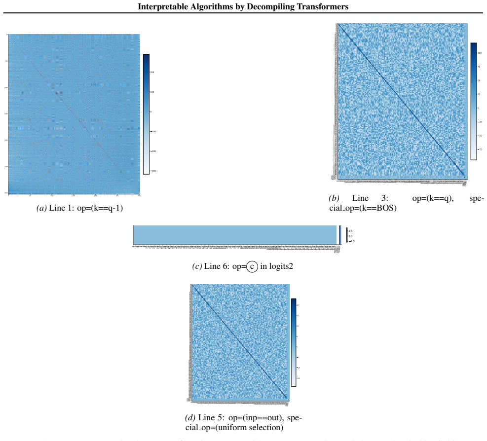
prediction = softmax(logits1+ logits2) InterpretationThis is discussed in Main paper, Figure 3. 72 Interpretable Algorithms by Decompiling Transformers 0 50 100 150 200 250 300 0 50 100 150 200 250 300 0 2000 4000 6000 8000 10000 (a) Line 1: op=(k==q-1) 01234567891011121314151...
2000
-
[163]
s2 = select(q=pos, k=pos, op= b ) # layer 0 head 0
-
[164]
s3 = select(k=token, op= d )
-
[165]
s4 = select(k=pos, op= e )
-
[166]
a1 = aggregate(s=s1+s2+s3+s4, v=token) # layer 0 head 0
-
[167]
s5 = select(q=token, k=token, op=(k==q), special op=(k==SEP)) # layer 1 head 0
-
[168]
a2 = aggregate(s=s5, v=a1) # layer 1 head 0
-
[169]
logits1 = project(inp=a2, op= f )
-
[170]
(Figure 58a)
prediction = softmax(logits1) InterpretationLine 1 defines a selector that assigns increased weight to SEP, with strength varying with the query. (Figure 58a). Line 2 defines a selector assigning increased weight to the immediately preceding position (Figure 58b). Line 3 defin...
2000
-
[171]
s1 = select(q=pos, k=pos, op= a ) # layer 0 head 0
-
[172]
s2 = select(k=token, op= d )
-
[173]
a1 = aggregate(s=s1+s2, v=token) # layer 0 head 0
-
[174]
s3 = select(q=token, k=token, op=(k==q), special op=(uniform selection)) # layer 2 head 0
-
[175]
s4 = select(q=token, k=a1, op= c ) # layer 2 head 0
-
[176]
a2 = aggregate(s=s3+s4, v=a1) # layer 2 head 0
-
[177]
new_a2 = element_wise_op(a2) # layer 3 mlp
-
[178]
logits1 = project(inp=new_a2, op=(inp==out))
-
[179]
s1 defines a selector that looks at the previous token in the input string, and s2 puts increased attention on SEP (Figure 60a,d)
prediction = softmax(logits1) InterpretationComparing the activations in Figure 61 with those of the other program on the same task (Figure 59) shows some commonalities, and indeed the algorithm is similar. s1 defines a selector that looks at the previous token in the input st...
2000
-
[181]
a2 = aggregate(s=[], v=pos) # layer 0 head 0
-
[182]
s1 = select(q=token, k=token, op= a ) # layer 0 head 1
-
[183]
s2 = select(q=pos, k=token, op= c ) # layer 0 head 1
-
[184]
s3 = select(k=token, op= b )
-
[185]
a3 = aggregate(s=s1+s2+s3, v=token) # layer 0 head 1
-
[186]
a4 = aggregate(s=s1+s2+s3, v=pos) # layer 0 head 1
-
[188]
new_a3 = element_wise_op(a3) # layer 0 mlp
-
[190]
logits2 = project(inp=a2, op= d )
-
[191]
logits3 = project(inp=new_a3, op=(inp==out))
-
[192]
logits4 = project(inp=a4, op= e )
-
[193]
imperfections
prediction = sigmoid(logits1+ logits2+ logits3+ logits4) InterpretationThis program is a more complex version of the D4 program discussed in the main paper Figure 8. Similar to Figure 8, a1 aggregates all the tokens in the input string, and then feeds into the MLP in Line 8, w...
-
[197]
logits1 = project(inp=token, op= b )
-
[198]
logits2 = project(inp=a1, op= c )
-
[199]
logits3 = project(inp=token, op= d )
-
[200]
logits4 = project(inp=new_a1, op=(inp==out))
-
[201]
logits5 = project(op= e )
-
[202]
a” and “b
prediction = sigmoid(logits1+ logits2+ logits3+ 89 Interpretable Algorithms by Decompiling Transformers logits4+ logits5) InterpretationThis program is a more complex version of the D4 program discussed in Figure 8 the main paper. Of note, the selector in Line 1 assigns unequa...
2023
-
[203]
a1 = aggregate(s=[], v=token) # layer 0 head 0
-
[204]
new_a1 = element_wise_op(a1) # layer 0 mlp
-
[205]
logits1 = project(inp=new_a1, op=(inp==out))
-
[206]
a” is allowed as long as the depth doesn’t exceed 4; “EOS
prediction = sigmoid(logits1) InterpretationThis program is discussed in the main paper, Figure 8. We provide further examples of the elementwise operation below. <bos> a a a a b b b b <eos> a b <bos> <sep> <eos> <pad> 0.0 0.2 0.4 0.6 0.8 1.0 (a) Line 1: a1 <bos> a a a a b b b...
-
[207]
s1 = select(k=token, op=(k==BOS))
-
[208]
a1 = aggregate(s=s1, v=pos) # layer 0 head 1
-
[209]
m1 = element_wise_op(pos+a1) # layer 0 mlp
-
[210]
logits1 = project(inp=m1, op=(inp==out))
-
[211]
Line 3 now jointly processes the current position with the position of BOS in an elementwise operation
prediction = sigmoid(logits1) InterpretationLines 1–2 retrieve the position of BOS (note that, while the position is 0 in this example, this does not generally hold due to the use of random offsets in positional encoding during training). Line 3 now jointly processes the curre...
-
[213]
a b c d e <bos><sep><eos><pad> a b c d e <bos> <sep> <eos> <pad> 10 5 0 5 (a) Line 1: op= a in logits1 Figure 85.Heatmaps supporting the program for abcde model
prediction = sigmoid(logits1) InterpretationThis program is discussed in the main paper. a b c d e <bos><sep><eos><pad> a b c d e <bos> <sep> <eos> <pad> 10 5 0 5 (a) Line 1: op= a in logits1 Figure 85.Heatmaps supporting the program for abcde model. <bos> a b c d d d d e <eos...
-
[214]
s1 = select(k=token, op= b )
-
[215]
a1 = aggregate(s=s1, v=token) # layer 0 head 0 97 Interpretable Algorithms by Decompiling Transformers
-
[216]
logits1 = project(inp=a1, op= a )
-
[217]
logits2 = project(op= c )
-
[218]
d” has occurred so far: if it hasn’t, {a, b, d}are valid; if it has, {b, c, EOS}are valid. Indeed, lines 1–2 encode this information by assigning weight to “d
prediction = sigmoid(logits1+ logits2) InterpretationEssentially, the model needs to check if “d” has occurred so far: if it hasn’t, {a, b, d}are valid; if it has, {b, c, EOS}are valid. Indeed, lines 1–2 encode this information by assigning weight to “d” if it has occurred. Li...
-
[219]
prediction = sigmoid(bias) K.8. tomita2 Task Description: ⟨bos⟩(10) ∗ ⟨eos⟩ Architecture:Layers: 1 Heads: 1 Hidden Dim: 16 LR: 0.001 Dropout: 0 Performance (w/Pruning→w/Primitives):Task Accuracy:1.00→1.00; Match Accuracy:1.00→1.00 Code
-
[220]
logits1 = project(inp=token, op= a )
-
[221]
prediction = sigmoid(logits1) InterpretationThis program straightforwardly describes next-token expectations in terms of the current token: BOS is followed by 1 or EOS; 1 is followed by 0; 0 is followed by 1 or EOS. 99 Interpretable Algorithms by Decompiling Transformers 0 1 <...
-
[222]
s1 = select(q=token, k=token, op= a ) # layer 0 head 0
-
[223]
a1 = aggregate(s=s1, v=token) # layer 0 head 0
-
[224]
s2 = select(q=token, k=a1, op=(k==q), special op=(uniform selection)) # layer 1 head 0
-
[225]
a2 = aggregate(s=s2, v=a1) # layer 1 head 0
-
[226]
logits1 = project(inp=a2, op= c )
-
[227]
logits2 = project(op= d )
-
[228]
In s1 (Figure 91a) q=0 pays attention to 1’s and q=1 to 0’s, and thus a1 (Figure 92b) holds the count of 0’s (for q=1) and 1’s (for q=0) before the current token
prediction = sigmoid(logits1+ logits2) InterpretationThe model essentially prohibits generating a 0 if a 1∗0∗1∗ subsequence is detected in Lines 1-4. In s1 (Figure 91a) q=0 pays attention to 1’s and q=1 to 0’s, and thus a1 (Figure 92b) holds the count of 0’s (for q=1) and 1’s ...
2000
-
[2020]
emnlp-main.576/
URL https://aclanthology.org/2020. emnlp-main.576/. Butoi, A., Khalighinejad, G., Svete, A., Valvoda, J., Cot- terell, R., and DuSell, B. Training neural networks as recognizers of formal languages. InThe Thirteenth Inter- national Conference on Learning Representations, Sin- ...
2020
-
[2021]
Most Frequent
URL https://aclanthology.org/2021. acl-long.292/. Yin, K. and Steinhardt, J. Which attention heads matter for in-context learning? InForty-second International Conference on Machine Learning, 2025. URL https: //openreview.net/forum?id=C7XmEByCFv. Zhang, Y ., Bi, W., Zhang, K.,...
2021 arXiv
-
[2022]
acl-long.527/
URL https://aclanthology.org/2022. acl-long.527/. Conmy, A., Mavor-Parker, A., Lynch, A., Heimersheim, S., and Garriga-Alonso, A. Towards automated circuit discovery for mechanistic interpretability.Advances in Neural Information Processing Systems, 36:16318– 16352, 2023. URL ...
2022
-
[2023]
io/Inverse_Tracr.pdf
URL https://william-baker.github. io/Inverse_Tracr.pdf. Baroni, L., Khara, G., Schaeffer, J., Subkhankulov, M., and Heimersheim, S. Transformers don’t need LayerNorm at inference time: Scaling LayerNorm removal to GPT-2 XL and the implications for mechanistic interpretability....
2025 arXiv
-
[2024]
Bhattamishra, S., Ahuja, K., and Goyal, N
URL https://openreview.net/forum? id=8oSY3rA9jY. Bhattamishra, S., Ahuja, K., and Goyal, N. On the ability and limitations of transformers to rec- ognize formal languages. InProceedings of the 2020 Conference on Empirical Methods in Natu- ral Language Processing (EMNLP), pp. 7...
2020
-
[2025]
Lai-Dang, Q.-V ., Kang, T., and Son, S
URL https://openreview.net/forum? id=Huw15LqglI. Lai-Dang, Q.-V ., Kang, T., and Son, S. Adaptive trans- former programs: Bridging the gap between performance and interpretability in transformers. InThe Thirteenth International Conference on Learning Representations,
Reviewed August 3, 2026 · model on record in the stance chip above.
Discussion (0). Continue with ORCID to comment.