Recognition: no theorem link
TreeGrad-Ranker: Feature Ranking via O(L)-Time Gradients for Decision Trees
Pith reviewed 2026-05-16 02:35 UTC · model grok-4.3
The pith
Feature rankings for decision trees come from directly optimizing a joint insertion-deletion objective with O(L)-time gradients.
A machine-rendered reading of the paper's core claim, the machinery that carries it, and where it could break.
Core claim
TreeGrad computes the gradients of the multilinear extension of the joint objective in O(L) time for decision trees with L leaves; these gradients include weighted Banzhaf values. TreeGrad-Ranker then aggregates the gradients while optimizing the joint objective to produce feature rankings.
What carries the argument
TreeGrad, the algorithm that evaluates gradients of the multilinear extension of the joint objective in O(L) time.
If this is right
- TreeGrad-Ranker feature rankings will be significantly better on insertion and deletion metrics than those from probabilistic values.
- Feature scores from TreeGrad-Ranker will satisfy all axioms uniquely characterizing probabilistic values except linearity.
- TreeGrad-Shap will compute Beta Shapley values with integral parameters in a numerically stable manner.
- TreeProb will generalize Linear TreeShap to support computation of all probabilistic values.
Where Pith is reading between the lines
- If the approach generalizes, similar gradient-based optimization could improve feature attribution for other model families.
- The O(L) scaling opens the possibility of using joint-objective rankings on very deep or wide trees.
- Excluding linearity may allow new ranking methods that trade off some axiomatic properties for practical performance.
Load-bearing premise
That directly optimizing the joint insertion-deletion objective on the multilinear extension yields feature rankings that are more useful in practice than those produced by probabilistic values, even though the paper shows the latter are theoretically unreliable for the same objective.
What would settle it
An experiment on a standard benchmark dataset where TreeGrad-Ranker rankings produce worse insertion or deletion curves than rankings based on Shapley values.
Figures


read the original abstract
We revisit the use of probabilistic values, which include the well-known Shapley and Banzhaf values, to rank features for explaining the local predicted values of decision trees. The quality of feature rankings is typically assessed with the insertion and deletion metrics. Empirically, we observe that co-optimizing these two metrics is closely related to a joint optimization that selects a subset of features to maximize the local predicted value while minimizing it for the complement. However, we theoretically show that probabilistic values are generally unreliable for solving this joint optimization. Therefore, we explore deriving feature rankings by directly optimizing the joint objective. As the backbone, we propose TreeGrad, which computes the gradients of the multilinear extension of the joint objective in $O(L)$ time for decision trees with $L$ leaves; these gradients include weighted Banzhaf values. Building upon TreeGrad, we introduce TreeGrad-Ranker, which aggregates the gradients while optimizing the joint objective to produce feature rankings, and TreeGrad-Shap, a numerically stable algorithm for computing Beta Shapley values with integral parameters. In particular, the feature scores computed by TreeGrad-Ranker satisfy all the axioms uniquely characterizing probabilistic values, except for linearity, which itself leads to the established unreliability. Empirically, we demonstrate that the numerical error of Linear TreeShap can be up to $10^{15}$ times larger than that of TreeGrad-Shap when computing the Shapley value. As a by-product, we also develop TreeProb, which generalizes Linear TreeShap to support all probabilistic values. In our experiments, TreeGrad-Ranker performs significantly better on both insertion and deletion metrics. Our code is available at https://github.com/watml/TreeGrad.
Editorial analysis
A structured set of objections, weighed in public.
Referee Report
Summary. The paper argues that probabilistic values (Shapley, Banzhaf) are theoretically unreliable for jointly optimizing insertion and deletion metrics in local feature ranking for decision trees. It introduces TreeGrad, an O(L)-time algorithm to compute gradients of the multilinear extension of this joint objective (including weighted Banzhaf values), TreeGrad-Ranker that aggregates the gradients to produce rankings, and TreeGrad-Shap for numerically stable Beta Shapley values with integral parameters. TreeProb generalizes Linear TreeShap to all probabilistic values. Experiments claim TreeGrad-Ranker outperforms baselines on insertion/deletion curves, with code released.
Significance. If the central claims hold, the work supplies a computationally efficient, direct-optimization route to feature rankings that aligns with the insertion/deletion evaluation protocol, together with a clean separation from the axiomatic limitations of probabilistic values. The O(L) gradient routine, numerical-stability improvement over Linear TreeShap (up to 10^15 factor), and supplied code are concrete strengths that would be useful for practitioners working with tree ensembles.
minor comments (1)
- [Experiments] The experimental section claims that TreeGrad-Ranker 'performs significantly better' on insertion and deletion metrics, yet reports neither variance across random seeds nor statistical significance tests. Including these would make the empirical superiority claim more robust.
Simulated Author's Rebuttal
We thank the referee for the positive summary of our manuscript, the recognition of its significance, and the recommendation for minor revision. We are pleased that the core contributions—the O(L)-time gradients via the multilinear extension, the direct optimization route for insertion/deletion alignment, the numerical stability improvement, and the clean separation from probabilistic-value axioms—are viewed as strengths. No major comments were raised in the report.
Circularity Check
No significant circularity in derivation chain
full rationale
The central derivation computes gradients of the multilinear extension of the joint insertion-deletion objective directly via standard calculus on the tree structure, yielding an O(L) algorithm whose output (including weighted Banzhaf values) is not defined in terms of itself or fitted to the target rankings. The theoretical unreliability result for probabilistic values is proven separately and does not rely on the new gradients. TreeGrad-Ranker aggregates these gradients while optimizing the objective; this step is algorithmic rather than tautological. No load-bearing self-citations, ansatzes smuggled via prior work, or renaming of known results appear in the derivation. The method is self-contained and externally falsifiable via the supplied code and insertion/deletion metrics.
Axiom & Free-Parameter Ledger
axioms (1)
- standard math Multilinear extension of set functions
Forward citations
Cited by 1 Pith paper
-
WOODELF-HD: Efficient Background SHAP for High-Depth Decision Trees
WoodelfHD reduces Background SHAP preprocessing for decision trees from 3^D to 2^D complexity, enabling exact computation on depths up to 21 with reported speedups of 33x to 162x.
Reference graph
Works this paper leans on
-
[1]
11 Published as a conference paper at ICLR 2026 Diederik P. Kingma and Jimmy Ba. Adam: A method for stochastic optimization. InProceedings of the 3rd International Conference on Learning Representations,
work page 2026
-
[2]
RISE: Randomized Input Sampling for Explanation of Black-box Models
Vitali Petsiuk, Abir Das, and Kate Saenko. Rise: Randomized input sampling for explanation of black-box models.arXiv preprint arXiv:1806.07421,
work page internal anchor Pith review Pith/arXiv arXiv
-
[3]
A value for n-person games.Annals of Mathematics Studies, 28:307–317,
12 Published as a conference paper at ICLR 2026 Lloyd S Shapley. A value for n-person games.Annals of Mathematics Studies, 28:307–317,
work page 2026
-
[4]
13 Published as a conference paper at ICLR 2026 Table of Contents A Semi-Values 14 B Polynomial Manipulations in Linear TreeShap 15 C Implementation of TreeProb 15 D How to Evolve Linear TreeShap into TreeShap-K 16 E One MoreO(LD)-Time andO(D 2+L)-Space Algorithm for Computing the Shapley Value 17 F Missing Proofs 19 G Experiments 24 A SEMI-VALUES One pop...
work page 2026
-
[5]
(10) Therefore,ϕ µ(fx)is used to denote semi-values
Besides,ϕ ω is a semi-value if and only if there exists a Borel probability measureµover the closed interval[0,1]such that for everyk∈[N] ωk = Z 1 0 tk−1(1−t) N−k dµ(t). (10) Therefore,ϕ µ(fx)is used to denote semi-values. Ifµis some Dirac measureδ ν, the resulting semi- value is a weighted Banzhaf value parameterized byν∈[0,1]. Ifµ(A)∝ R A zβ−1(1−z) α−1d...
work page 2026
-
[6]
to generate feature scores. B POLYNOMIALMANIPULATIONS INLINEARTREESHAP In manipulating polynomials, the most expensive step is the multiplication ofp(y)and(1 + y)d−deg(p), the degree of each is at mostDin the context. In general, polynomial multiplication re- quiresO(DlogD)time to compute using fast Fourier transform (Cormen et al., 2022, Chapter 30), whi...
work page 2022
-
[7]
Upon reaching a leaf (line 46), Linear TreeShap computesp(y)← ϱvcv cr ·p(y). In line 48, it performs pa(y)←traverse(a v, p(y)), p b(y)←traverse(b v, p(y)), d max ←max(deg(p a(y)),deg(p b(y))) p(y)←p a(y)·(1 +y) dmax−deg(pa(y)) +p b(y)·(1 +y) dmax−deg(pb(y)) As a result, when evaluatingψin line 52, the degree ofG[v]is not fixed, and may vary from1to D. Con...
work page 2026
-
[8]
One may think that the space com- plexityO(LD). We remark that there are onlyO(D)polynomials that are needed on the spot and thus the complexity isO(D 2+L). Therefore, for computing probabilistic values, the time and space complexities of TreeProb areO(LD)andO(D 2 +L), respectively. D HOW TOEVOLVELINEARTREESHAP INTOTREESHAP-K How to avoid the use of Vande...
work page 2026
-
[9]
Then, ϱvcv cr ·θ |Pv| = ϑv. What TreeShap-K computes in the traversing-up procedure is ϕShap i (fx) = X e∈E le=i (γe −1)·sum( X v∈L† he ϑv ⊖γ e) wheresumsimply adds up all the entries. All in all, TreeShap-K proposed by Karczmarz et al. (2022, Appendix E) is summarized in Algorithm
work page 2022
-
[10]
Indeed, the substantial inaccuracy of TreeShap-K is already confirmed by Karczmarz et al
We point out that the⊖operation essentially involves solving a linear equation, whose condition number, as shown in Figure 2, grows expo- nentially w.r.t.D(withγset to1). Indeed, the substantial inaccuracy of TreeShap-K is already confirmed by Karczmarz et al. (2022, Figure 1). E ONEMOREO(LD)-TIME ANDO(D 2 +L)-SPACEALGORITHM FOR COMPUTING THESHAPLEYVALUE ...
work page 2022
-
[11]
However, its numerical error still blows up, which we suspect is due to the repeated use of⊟. F MISSINGPROOFS Proposition 2.Letπbe a ranking induced by a probabilistic valueϕ ω(fx)such thatϕ ω π(1)(fx)≥ ϕω π(2)(fx)≥ · · · ≥ϕ ω π(N) (fx). For every1≤k≤N,S + k :={π(1), π(2), . . . , π(k)}is an optimal solution to the problem maximize S⊆[N],|S|=k 1 2 (g∗(S)−...
work page 2026
-
[12]
LetU: 2 [N] →Rbe a utility function and denote byGthe set that contains all such utility functions
Moreover, it verifies the axioms of dummy, equal treatment and monotonic- ity. LetU: 2 [N] →Rbe a utility function and denote byGthe set that contains all such utility functions. The axioms of interest are listed in the below. 1.Linearity:ϕ(c·U+U ′) =c·ϕ(U) +ϕ(U ′)for everyU, U ′ ∈ Gandc∈R. 2.Equal Treatment: For somei, j∈[N], ifU(S∪i) =U(S∪j)for everyS⊆[...
work page 2026
-
[13]
Suppose there exist a featurei∈[N]and a constantC∈Rsuch thatf x(S∪i) = fx(S) +Cfor everyS⊆[N]\i
The dependence ofxcomes from that different instances ofxwould induce different trajectories along which the gradients are accumulated and averaged. Suppose there exist a featurei∈[N]and a constantC∈Rsuch thatf x(S∪i) = fx(S) +Cfor everyS⊆[N]\i. In this case, ∇if x(z) =C· X S⊆[N]\i ωi(S) =Cfor everyz∈[0,1] N . On average, it is clear thatζ i =C. Therefore...
work page 2026
-
[14]
Without vectorization (Algorithm 6), its space complexity isO(L)
computes Beta Shapley value with integral parameters usingO(LD)time andO(D 2 +L)space. Without vectorization (Algorithm 6), its space complexity isO(L). Proof.By linearity and (Dubey et al., 1981, Theorem 1(a ′)), ϕShap(fx) = Z 1 0 ∇f x(t·1 N)dt= Z 1 0 X v∈Lr ∇R v x(t·1 N)dt Using Eq. (7), ∇iR v x(t·1 N) = X S⊆[N]\i ts(1−t) N−1−s[Rv x(S∪i)−R v x(S)], whic...
work page 1981
-
[15]
Therefore, we have f x(z)< f ∗
=U ∗, which contradicts the assumption thatS ∗ is unique. Therefore, we have f x(z)< f ∗. 22 Published as a conference paper at ICLR 2026 Algorithm 6TreeGrad-Shap Input:Decision treeT= (V, E)with rootrand depthD, instancex∈R N , integral parameter (α, β)that specifies some Beta Shaple value Output:Shapley valueϕ 90Initializeϕ=0 N 91M←min(D, N) +α+β−2 92Ge...
work page 2026
-
[16]
Our TreeGrad-Ranker also works for gradient boosted trees (Friedman, 2001). We train gradient boosted trees on the same datasets using GradientBoostingClassifier and GradientBoostingRegres- sor from the scikit-learn library. The corresponding results are presented in Figures 9–13. For classification tasks, the output of each gradient boosted trees model i...
work page 2001
-
[17]
149z←z+ϵ· ˆmt/√ˆvt +ϵ ′ 150z←Proj(z)//z i ←min(max(0, z i),1) 151returnζ Table 1: Summary of the datasets used in this work. Dataset #Instances #Features Link Task #Classes FOTP (Bridge et al., 2014)6,118 51https://openml.org/d/1475classification6 GPSP (Madeo et al., 2013)9,873 32https://openml.org/d/4538classification5 jannis83,733 54https://openml.org/d...
work page 2014
-
[18]
8https://github.com/yupbank/linear_tree_shap/blob/main/linear_tree_ shap/fast_linear_tree_shap.py
7https://openml.org/d/1219. 8https://github.com/yupbank/linear_tree_shap/blob/main/linear_tree_ shap/fast_linear_tree_shap.py. 9https://github.com/shap/shap. 25 Published as a conference paper at ICLR 2026 Table 2: The sizes of the trained tree models and their performance on the test datasets. We report test accuracy for classification tasks and the coef...
work page 2026
-
[19]
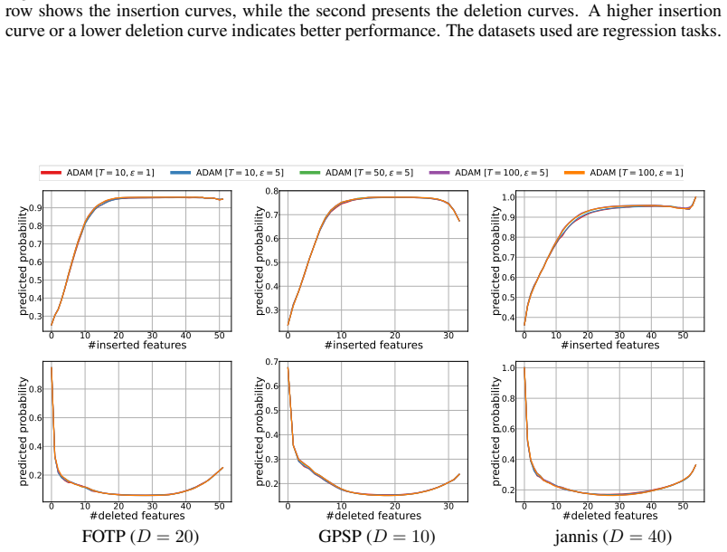
Next, using decision trees, we present the performance across different combi- nations ofTandϵ. The results obtained with gradient ascent are shown in Figures 14–18, whereas those for ADAM are presented in Figures 19–23. Our observations are: (i) the resulting performance improves and converges asTincreases; (ii) TreeGrad-Ranker with ADAM converges earlie...
work page 2026
-
[20]
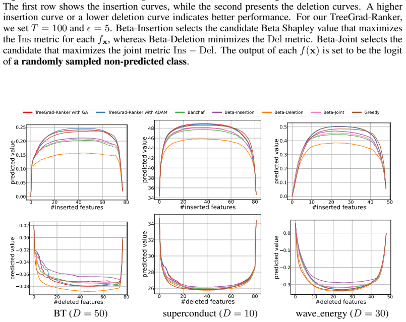
Beta-Joint selects the candidate that maximizes the joint metricIns−Del
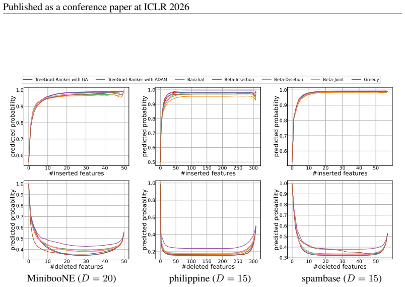
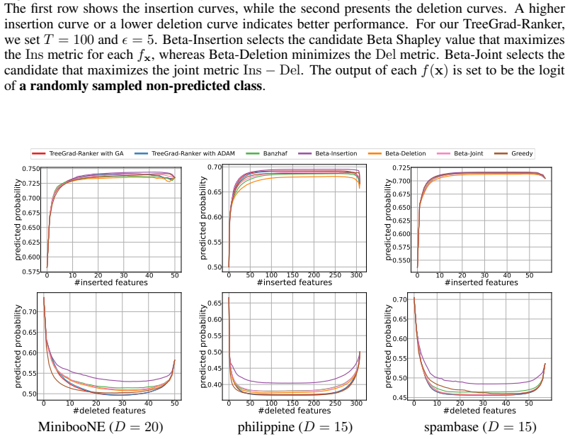
Beta-Insertion selects the candidate Beta Shapley value that maximizes theInsmetric for eachf x, whereas Beta-Deletion minimizes theDelmetric. Beta-Joint selects the candidate that maximizes the joint metricIns−Del. The output of eachf(x)is set to be the probability ofa randomly sampled non-predicted class. 28 Published as a conference paper at ICLR 2026 ...
work page 2026
-
[21]
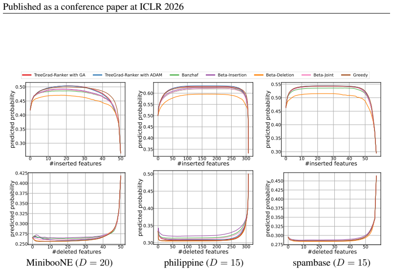
Beta-Joint selects the candidate that maximizes the joint metricIns−Del
Beta-Insertion selects the candidate Beta Shapley value that maximizes theInsmetric for eachf x, whereas Beta-Deletion minimizes theDelmetric. Beta-Joint selects the candidate that maximizes the joint metricIns−Del. The output of eachf(x)is set to be the logit ofits predicted class. 29 Published as a conference paper at ICLR 2026 0.04 0.02 0.00 0.02 0.04 ...
work page 2026
-
[22]
Beta-Joint selects the candidate that maximizes the joint metricIns−Del
Beta-Insertion selects the candidate Beta Shapley value that maximizes theInsmetric for eachf x, whereas Beta-Deletion minimizes theDelmetric. Beta-Joint selects the candidate that maximizes the joint metricIns−Del. The output of eachf(x)is set to be the logit ofits predicted class. 30 Published as a conference paper at ICLR 2026 0.04 0.02 0.00 0.02 0.04 ...
work page 2026
-
[23]
Beta-Joint selects the candidate that maximizes the joint metricIns−Del
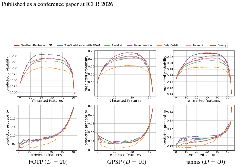
Beta-Insertion selects the candidate Beta Shapley value that maximizes theInsmetric for eachf x, whereas Beta-Deletion minimizes theDelmetric. Beta-Joint selects the candidate that maximizes the joint metricIns−Del. The datasets used are regression tasks. 31 Published as a conference paper at ICLR 2026 0.04 0.02 0.00 0.02 0.04 0.04 0.02 0.00 0.02 0.04 GA ...
work page 2026
-
[24]
All trained models aredecision trees
Figure 15: Results of TreeGrad-Ranker withGA. All trained models aredecision trees. The first row shows the insertion curves, while the second presents the deletion curves. A higher insertion curve or a lower deletion curve indicates better performance. The output of eachf(x)is set to be the probability ofa randomly sampled non-predicted class. 32 Publish...
work page 2026
-
[25]
All trained models aredecision trees
Figure 17: Results of TreeGrad-Ranker withGA. All trained models aredecision trees. The first row shows the insertion curves, while the second presents the deletion curves. A higher insertion curve or a lower deletion curve indicates better performance. The output of eachf(x)is set to be the probability ofa randomly sampled non-predicted class. 33 Publish...
work page 2026
-
[26]
All trained models aredecision trees
Figure 19: Results of TreeGrad-Ranker withADAM. All trained models aredecision trees. The first row shows the insertion curves, while the second presents the deletion curves. A higher insertion curve or a lower deletion curve indicates better performance. The output of eachf(x)is set to be the probability ofits predicted class. 34 Published as a conferenc...
work page 2026
-
[27]
All trained models aredecision trees
Figure 21: Results of TreeGrad-Ranker withADAM. All trained models aredecision trees. The first row shows the insertion curves, while the second presents the deletion curves. A higher insertion curve or a lower deletion curve indicates better performance. The output of eachf(x)is set to be the probability ofits predicted class. 35 Published as a conferenc...
work page 2026
discussion (0)
Sign in with ORCID, Apple, or X to comment. Anyone can read and Pith papers without signing in.