Recognition: 1 theorem link
· Lean TheoremSolving Inverse Parametrized Problems via Finite Elements and Extreme Learning Networks
Pith reviewed 2026-05-15 21:55 UTC · model grok-4.3
The pith
Finite element spatial discretization paired with extreme learning machine parameter surrogates solves inverse parametrized PDE problems with explicit error estimates.
A machine-rendered reading of the paper's core claim, the machinery that carries it, and where it could break.
Core claim
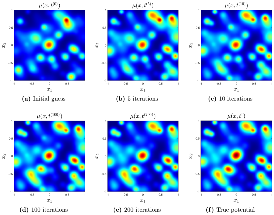
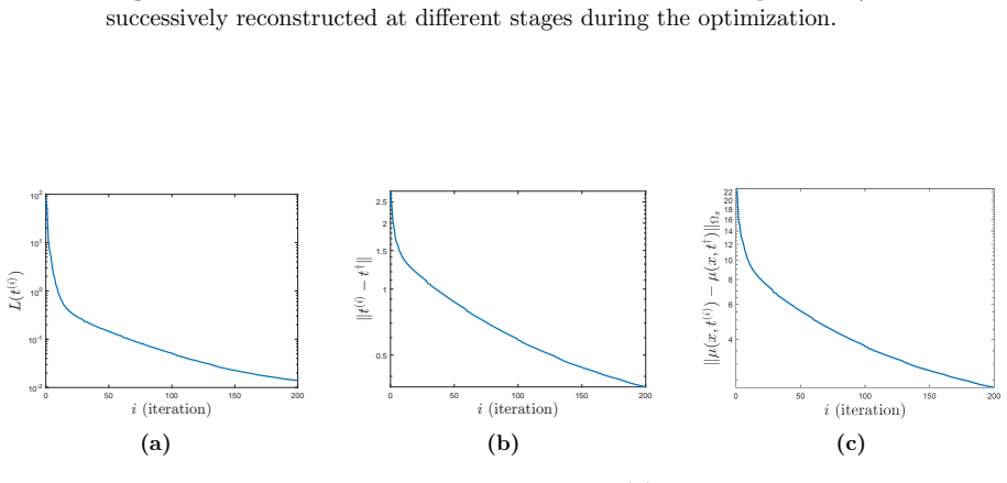
We establish existence, uniqueness, and regularity of the parametric solution and derive rigorous error estimates that explicitly quantify the interplay between spatial discretization and parameter approximation. In low-dimensional parameter spaces, classical interpolation schemes yield algebraic convergence rates based on Sobolev regularity in the parameter variable. In higher-dimensional parameter spaces, we replace classical interpolation by extreme learning machine (ELM) surrogates and obtain error bounds under explicit approximation and stability assumptions. The proposed framework is applied to inverse problems in quantitative photoacoustic tomography, where we derive potential and 1.0
What carries the argument
The interpolation-based modeling framework that separates finite-element spatial discretization from parameter approximation performed either by classical interpolation or by extreme learning machine surrogates.
Load-bearing premise
Error bounds in higher-dimensional parameter spaces require explicit approximation and stability assumptions on the extreme learning machine surrogates.
What would settle it
A numerical test in quantitative photoacoustic tomography in which the observed reconstruction error for a chosen mesh size and ELM surrogate exceeds the theoretically derived bound for that discretization pair would falsify the error estimates.
Figures


read the original abstract
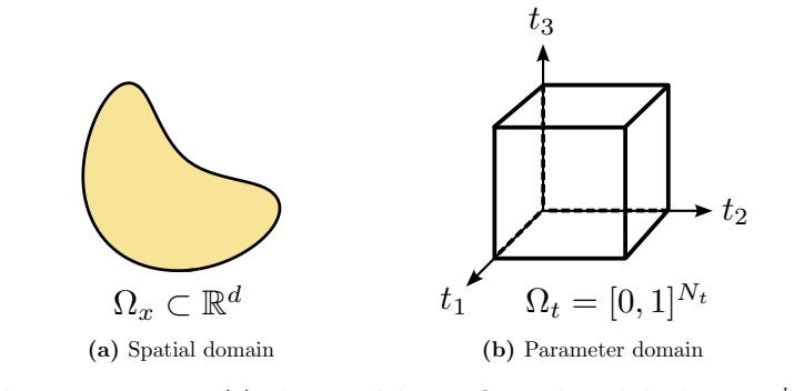
We develop an interpolation-based modeling framework for parameter-dependent partial differential equations arising in control, inverse problems, and uncertainty quantification. The solution is discretized in the physical domain using finite element methods, while the dependence on a finite-dimensional parameter is approximated separately. We establish existence, uniqueness, and regularity of the parametric solution and derive rigorous error estimates that explicitly quantify the interplay between spatial discretization and parameter approximation. In low-dimensional parameter spaces, classical interpolation schemes yield algebraic convergence rates based on Sobolev regularity in the parameter variable. In higher-dimensional parameter spaces, we replace classical interpolation by extreme learning machine (ELM) surrogates and obtain error bounds under explicit approximation and stability assumptions. The proposed framework is applied to inverse problems in quantitative photoacoustic tomography, where we derive potential and parameter reconstruction error estimates and demonstrate substantial computational savings compared to standard approaches, without sacrificing accuracy.
Editorial analysis
A structured set of objections, weighed in public.
Referee Report
Summary. The paper develops an interpolation-based modeling framework for parameter-dependent PDEs, using finite element discretization in the physical domain and separate approximation of the parameter dependence. It establishes existence, uniqueness, and regularity of the parametric solution, derives rigorous error estimates quantifying the interplay between spatial discretization and parameter approximation, and applies the framework to inverse problems in quantitative photoacoustic tomography, claiming computational savings without loss of accuracy. Low-dimensional cases use classical interpolation with Sobolev rates; high-dimensional cases employ ELM surrogates under explicit approximation and stability assumptions.
Significance. If the central claims hold, the work offers a structured approach to parametric inverse problems with explicit error control that separates spatial and parameter errors, potentially enabling scalable computations in high-dimensional settings via ELM while preserving rigor in applications such as photoacoustic tomography.
major comments (1)
- [Abstract / high-dimensional parameter approximation] The error estimates for high-dimensional parameter spaces (as stated in the abstract) are derived only under explicit approximation and stability assumptions on the ELM surrogates. These assumptions are not shown to follow from the PDE structure or verified numerically within the manuscript, rendering the claimed rigor for the high-dimensional regime conditional rather than self-contained.
Simulated Author's Rebuttal
We thank the referee for the careful review and constructive feedback on our manuscript. We address the major comment below and will incorporate revisions to strengthen the presentation of the high-dimensional results.
read point-by-point responses
-
Referee: [Abstract / high-dimensional parameter approximation] The error estimates for high-dimensional parameter spaces (as stated in the abstract) are derived only under explicit approximation and stability assumptions on the ELM surrogates. These assumptions are not shown to follow from the PDE structure or verified numerically within the manuscript, rendering the claimed rigor for the high-dimensional regime conditional rather than self-contained.
Authors: We appreciate the referee highlighting this point. The manuscript explicitly conditions the high-dimensional error estimates on approximation and stability assumptions for the ELM surrogates, as stated in the abstract and elaborated in the relevant theoretical sections. This is by design: the framework separates spatial FEM discretization from parameter-space approximation to remain modular and applicable to general parameter-dependent PDEs, with ELM serving as one possible surrogate in high dimensions. The assumptions are not derived from the specific PDE structure because they concern the general approximation theory of ELM networks, which is supported by prior literature on neural network surrogates. We agree, however, that the conditional nature merits clearer emphasis to prevent any perception of unconditional rigor. In the revised version we will (i) update the abstract to foreground the assumptions, (ii) add a concise discussion paragraph (with references to ELM approximation results) explaining when the assumptions are expected to hold for the photoacoustic tomography problem, and (iii) include targeted numerical checks of the stability and approximation quality on the concrete example. These changes will make the high-dimensional regime more self-contained while preserving the modular character of the framework. revision: yes
Circularity Check
Error estimates derived from discretization theory and stated ELM assumptions, no reduction to fitted inputs
full rationale
The paper's core claims rest on standard existence/uniqueness results for parametric PDEs, classical Sobolev interpolation rates for low-dimensional parameter spaces, and finite-element spatial error bounds. High-dimensional cases invoke ELM surrogates only under explicitly stated approximation and stability assumptions that are external to the derivation; these are not obtained by fitting parameters inside the paper's own equations and then relabeling them as predictions. No self-definitional loops, load-bearing self-citations, or ansatz smuggling appear in the derivation chain. The overall argument therefore remains self-contained against external benchmarks, warranting only a minor score for the conditional nature of the high-dimensional bounds.
Axiom & Free-Parameter Ledger
axioms (2)
- domain assumption Existence, uniqueness, and regularity of the parametric solution
- ad hoc to paper Explicit approximation and stability assumptions for ELM surrogates
Lean theorems connected to this paper
-
IndisputableMonolith/Foundation/RealityFromDistinction.leanreality_from_one_distinction unclear?
unclearRelation between the paper passage and the cited Recognition theorem.
We establish existence, uniqueness, and regularity of the parametric solution and derive rigorous error estimates that explicitly quantify the interplay between spatial discretization and parameter approximation.
What do these tags mean?
- matches
- The paper's claim is directly supported by a theorem in the formal canon.
- supports
- The theorem supports part of the paper's argument, but the paper may add assumptions or extra steps.
- extends
- The paper goes beyond the formal theorem; the theorem is a base layer rather than the whole result.
- uses
- The paper appears to rely on the theorem as machinery.
- contradicts
- The paper's claim conflicts with a theorem or certificate in the canon.
- unclear
- Pith found a possible connection, but the passage is too broad, indirect, or ambiguous to say the theorem truly supports the claim.
Reference graph
Works this paper leans on
-
[1]
G. S. Alberti, A. Arroyo, and M. Santacesaria. Inverse problems on low-dimensional manifolds. Nonlinearity, 36(1):734–808, 2023. doi:10.1088/1361-6544/aca73d
-
[2]
G. S. Alberti and M. Santacesaria. Calder´ on’s inverse problem with a finite number of measurements. Forum Math. Sigma, 7:Paper No. e35, 20, 2019. doi:10.1017/fms.2019.31
-
[3]
G. S. Alberti and M. Santacesaria. Infinite-dimensional inverse problems with finite measurements. Arch. Ration. Mech. Anal., 243(1):1–31, 2022. doi:10.1007/s00205-021-01718-4
-
[4]
G. Alessandrini, M. V. de Hoop, F. Faucher, R. Gaburro, and E. Sincich. Inverse problem for the Helmholtz equation with Cauchy data: reconstruction with conditional well-posedness driven iterative regularization.ESAIM Math. Model. Numer. Anal., 53(3):1005–1030, 2019. doi:10.1051/m2an/2019009
-
[5]
G. Alessandrini and S. Vessella. Lipschitz stability for the inverse conductivity problem.Adv. in Appl. Math., 35(2):207–241, 2005. doi:10.1016/j.aam.2004.12.002
-
[6]
S. R. Arridge. Optical tomography in medical imaging.Inverse Problems, 15(2):R41–R93, 1999. doi:10.1088/0266-5611/15/2/022. 40
-
[7]
S. R. Arridge and M. Schweiger. A general framework for iterative reconstruction algorithms in optical tomography, using a finite element method. InComputational radiology and imaging (Min- neapolis, MN, 1997), volume 110 ofIMA Vol. Math. Appl., pages 45–70. Springer, New York, 1999. doi:10.1007/978-1-4612-1550-9 4
-
[8]
G. Bal and K. Ren. Multi-source quantitative photoacoustic tomography in a diffusive regime. Inverse Problems, 27(7):075003, 20, 2011. doi:10.1088/0266-5611/27/7/075003
-
[9]
G. Bal and G. Uhlmann. Inverse diffusion theory of photoacoustics.Inverse Problems, 26(8):085010, 20, 2010. doi:10.1088/0266-5611/26/8/085010
-
[10]
A. R. Barron. Universal approximation bounds for superpositions of a sigmoidal function.IEEE Transactions on Information theory, 39(3):930–945, 1993
work page 1993
-
[11]
E. Burman, S. Cen, B. Jin, and Z. Zhou. Numerical approximation and analysis of the inverse Robin problem using the Kohn-Vogelius method.arXiv Preprint, 2025. doi:10.48550/arXiv.2506.07370
-
[12]
E. Burman, S. Claus, P. Hansbo, M. G. Larson, and A. Massing. CutFEM: discretizing geome- try and partial differential equations.Internat. J. Numer. Methods Engrg., 104(7):472–501, 2015. doi:10.1002/nme.4823
-
[13]
E. Burman, M. Kn¨ oller, and L. Oksanen. A computational method for the inverse Robin problem with convergence rate.arXiv Preprint, 2025. doi:10.48550/arXiv.2509.17571
-
[14]
E. Burman, M. G. Larson, K. Larsson, and C. Lundholm. Stabilizing and solving unique contin- uation problems by parameterizing data and learning finite element solution operators.Comput. Methods Appl. Mech. Engrg., 444:Paper No. 118111, 25, 2025. doi:10.1016/j.cma.2025.118111
-
[15]
E. Burman and L. Oksanen. Finite element approximation of unique continuation of func- tions with finite dimensional trace.Math. Models Methods Appl. Sci., 34(10):1809–1824, 2024. doi:10.1142/S0218202524500362
-
[16]
E. Burman, L. Oksanen, and Z. Zhao. Computational unique continuation with finite dimensional Neumann trace.SIAM J. Numer. Anal., 63(5):1986–2008, 2025. doi:10.1137/24M164080X
-
[17]
F. Calabro, G. Fabiani, and C. Siettos. Extreme learning machine collocation for the numeri- cal solution of elliptic PDEs with sharp gradients.Computer Methods in Applied Mechanics and Engineering, 387:114188, 2021. doi:10.1016/j.cma.2021.114188
-
[18]
G. Cybenko. Approximation by superpositions of a sigmoidal function.Mathematics of control, signals and systems, 2(4):303–314, 1989
work page 1989
-
[19]
V. Dwivedi and B. Srinivasan. Physics informed extreme learning machine (PIELM) – a rapid method for the numerical solution of partial differential equations.Neurocomputing, 391:96–118,
-
[20]
doi:10.1016/j.neucom.2019.12.017
-
[21]
V. Dwivedi and B. Srinivasan. A normal equation-based extreme learning machine for solving linear partial differential equations.Journal of Computing and Information Science in Engineering, 22:014502, 2022. doi:10.1115/1.4051556
-
[22]
H. Egger and B. Hofmann. Tikhonov regularization in Hilbert scales under conditional stability assumptions.Inverse Problems, 34(11):115015, 17, 2018. doi:10.1088/1361-6420/aadef4
-
[23]
H. W. Engl, M. Hanke, and A. Neubauer.Regularization of inverse problems, volume 375 of Mathematics and its Applications. Kluwer Academic Publishers Group, Dordrecht, 1996
work page 1996
-
[24]
L. C. Evans.Partial differential equations, volume 19 ofGraduate Studies in Mathematics. American Mathematical Society, Providence, RI, 1998. doi:10.1090/gsm/019
-
[25]
B. Harrach. Uniqueness, stability and global convergence for a discrete inverse elliptic Robin trans- mission problem.Numer. Math., 147(1):29–70, 2021. doi:10.1007/s00211-020-01162-8
-
[26]
J. S. Hesthaven, G. Rozza, and B. Stamm.Certified reduced basis methods for parametrized partial differential equations. SpringerBriefs in Mathematics. Springer, Cham; BCAM Basque Center for Applied Mathematics, Bilbao, 2016. doi:10.1007/978-3-319-22470-1. BCAM SpringerBriefs
-
[27]
G.-B. Huang, Q.-Y. Zhu, and C.-K. Siew. Extreme learning machine: a new learning scheme of feed- forward neural networks. In2004 IEEE International Joint Conference on Neural Networks (IEEE Cat. No.04CH37541), volume 2, pages 985–990 vol.2, 2004. doi:10.1109/IJCNN.2004.1380068. 41
-
[28]
G.-B. Huang, Q.-Y. Zhu, and C.-K. Siew. Extreme learning machine: Theory and applications. Neurocomputing, 70(1):489–501, 2006. doi:10.1016/j.neucom.2005.12.126. Neural Networks
-
[29]
K. Ito and B. Jin.Inverse problems: Tikhonov theory and algorithms, volume 22 ofSeries on Applied Mathematics. World Scientific Publishing Co. Pte. Ltd., Hackensack, NJ, 2015. doi:10.1142/9120
-
[30]
B. Jin, X. Lu, Q. Quan, and Z. Zhou. Convergence rate analysis of Galerkin approximation of inverse potential problem.Inverse Problems, 39(1):Paper No. 015008, 26, 2023. doi:10.1088/1361- 6420/aca70e
-
[31]
T. Jonsson, M. G. Larson, and K. Larsson. Cut finite element methods for elliptic problems on multipatch parametric surfaces.Comput. Methods Appl. Mech. Engrg., 324:366–394, 2017. doi:10.1016/j.cma.2017.06.018
-
[32]
M. V. Klibanov, J. Li, and W. Zhang. Convexification for an inverse parabolic problem.Inverse Problems, 36(8):085008, 32, 2020. doi:10.1088/1361-6420/ab9893
-
[33]
J. M. Klusowski and A. R. Barron. Risk bounds for high-dimensional ridge function combinations including neural networks.arXiv Preprint, 2016. doi:10.48550/arXiv.1607.01434
work page internal anchor Pith review Pith/arXiv arXiv doi:10.48550/arxiv.1607.01434 2016
-
[34]
Fourier Neural Operator for Parametric Partial Differential Equations
Z.-Y. Li et al. Fourier neural operator for parametric partial differential equations.arXiv, 2010.08895, 2020. doi:10.48550/arXiv.2010.08895
work page internal anchor Pith review Pith/arXiv arXiv doi:10.48550/arxiv.2010.08895 2010
- [35]
-
[36]
PMLR, 2020. doi:10.48550/arXiv.1908.10292
-
[37]
X. Liu, T. Mao, and J. Xu. Integral representations of Sobolev spaces via ReLU k acti- vation function and optimal error estimates for linearized networks.arXiv Preprint, 2025. doi:10.48550/arXiv.2505.00351
-
[38]
L. Lu, P. Jin, G. Pang, Z. Zhang, and G. E. Karniadakis. Learning nonlinear operators via DeepONet based on the universal approximation theorem of operators.Nature Machine Intelligence, 3:218–229,
-
[39]
doi:10.1038/s42256-021-00302-5
-
[40]
C. Ma, S. Wojtowytsch, L. Wu, et al. Towards a mathematical understanding of neural network- based machine learning: what we know and what we don’t.CSIAM Trans. Appl. Math., 1(4):561– 615, 2020. doi:10.4208/csiam-am.SO-2020-0002
-
[41]
C. Ma, L. Wu, et al. The generalization error of the minimum-norm solutions for over-parameterized neural networks.arXiv Preprint, 2019. doi:10.48550/arXiv.1912.06987
-
[42]
C. Ma, L. Wu, et al. The Barron space and the flow-induced function spaces for neural network models.Constructive Approximation, 55(1):369–406, 2022. doi:10.1007/s00365-021-09549-y
-
[43]
S. Panghal and M. Kumar. Optimization free neural network approach for solving ordinary and partial differential equations.Engineering with Computers, 37:2989–3002, 2021. doi:10.1007/s00366- 020-01209-4
-
[44]
A. Rangamani, L. Rosasco, and T. Poggio. For interpolating kernel machines, minimizing the norm of the ERM solution maximizes stability.Analysis and Applications, 21(01):193–215, 2023. doi:10.1142/S0219530522400115
-
[45]
A. R¨ uland and E. Sincich. On Runge approximation and Lipschitz stability for a finite-dimensional Schr¨ odinger inverse problem.Appl. Anal., 101(10):3655–3666, 2022. doi:10.1080/00036811.2020.1738403
-
[46]
T. D. Ryck, S. Mishra, Y. Shang, and F. Wang. Approximation theory and applications of randomized neural networks for solving high-dimensional PDEs.arXiv Preprint, 2025. doi:10.48550/arXiv.2501.12145
-
[47]
T. J. Santner, B. J. Williams, and W. I. Notz.The Design and Analysis of Computer Experiments. Springer, 2019. doi:10.1007/978-1-4757-3799-8
-
[48]
R. I. Saye. High-order quadrature methods for implicitly defined surfaces and volumes in hyper- rectangles.SIAM J. Sci. Comput., 37(2):A993–A1019, 2015. doi:10.1137/140966290. 42
-
[49]
E. Sincich. Lipschitz stability for the inverse Robin problem.Inverse Problems, 23(3):1311–1326,
-
[50]
doi:10.1088/0266-5611/23/3/027
-
[51]
T. Tarvainen and B. T. Cox. Quantitative photoacoustic tomography: modeling and inverse prob- lems.Journal of Biomedical Optics, 29(S1):S11509, 2023. doi:10.1117/1.JBO.29.S1.S11509
-
[52]
Y. Wang and S. Dong. An extreme learning machine-based method for computational PDEs in higher dimensions.Comput. Methods Appl. Mech. Engrg., 418:Paper No. 116578, 31, 2024. doi:10.1016/j.cma.2023.116578. Authors’ addresses: Erik Burman, Mathematics, University College London, UK e.burman@ucl.ac.uk Mats G. Larson, Mathematics and Mathematical Statistics, ...
discussion (0)
Sign in with ORCID, Apple, or X to comment. Anyone can read and Pith papers without signing in.