Recognition: 2 theorem links
· Lean TheoremMortality Forecasting as a Flow Field in Tucker Decomposition Space
Pith reviewed 2026-05-15 00:34 UTC · model grok-4.3
The pith
Mortality forecasting improves by integrating a flow field through the one-dimensional score space of a Tucker decomposition of historical data, producing lower bias than time-series methods.
A machine-rendered reading of the paper's core claim, the machinery that carries it, and where it could break.
Core claim
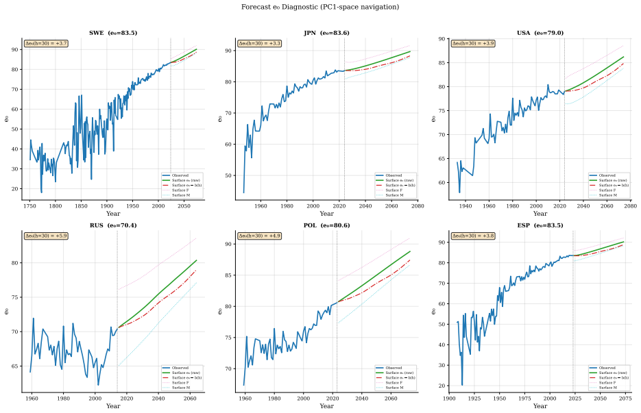
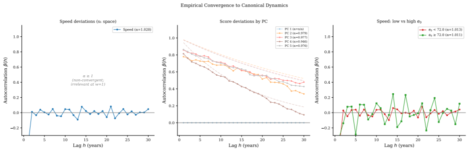
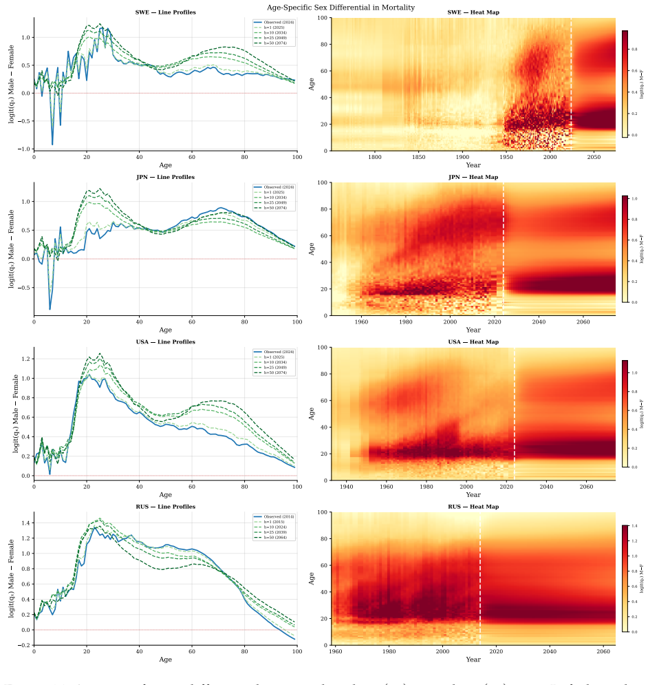
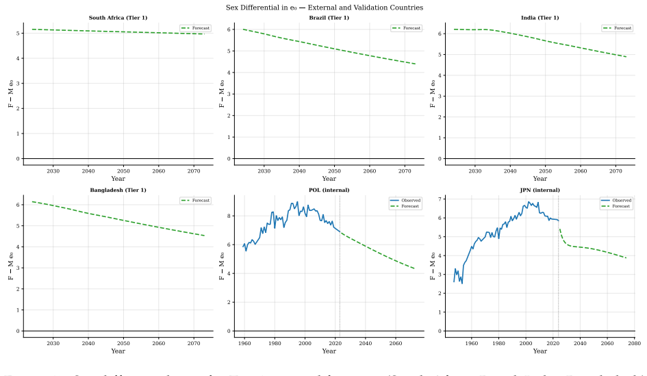
Mortality forecasting is reframed as integrating a flow field through the low-dimensional score space of a Tucker tensor decomposition of the Human Mortality Database; PCA reduction shows the mortality transition is essentially one-dimensional, parameterized by a scalar speed function that advances level and trajectory functions that supply structural scores, with Tucker reconstruction yielding complete sex-specific single-year-of-age mortality schedules at each horizon.
What carries the argument
The flow field on the PCA-reduced Tucker score space, where a scalar speed function advances mortality level and trajectory functions supply the structural scores for reconstruction.
If this is right
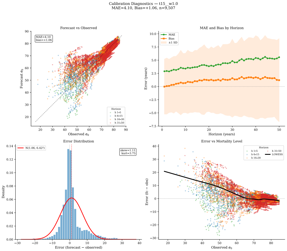
- Bias of only +1.058 years over 50-year horizons versus -3.2 years for Lee-Carter.
- 2.7 times lower error than the UN pipeline on 1.66 million sex-age-specific test points at every age and horizon.
- Complete age-specific schedules generated directly without separate model life tables.
- Navigation stays within observed mortality structures instead of extrapolating temporal trends.
Where Pith is reading between the lines
- Mortality schedules across populations may lie on a low-dimensional manifold traversable by simple flow rules.
- The same flow-field logic could be tested on fertility or cause-specific mortality data.
- Speed functions updated with recent observations might improve responsiveness to events like pandemics.
Load-bearing premise
The assumption that PCA reduction of the Tucker score space reveals the mortality transition to be essentially one-dimensional.
What would settle it
Future mortality data or held-out populations showing age-specific rates that deviate from the predicted one-dimensional trajectory in the Tucker score space.
Figures


read the original abstract
Mortality forecasting methods in the Lee-Carter tradition extrapolate temporal components via time-series models, often producing forecasts that systematically underpredict life expectancy at long horizons. This bias is consequential for planning pension funding, healthcare capacity, and social security solvency. The dominant alternative - the Bayesian double-logistic model underlying the UN World Population Prospects - forecasts scalar life expectancy and requires a separate model life table system to recover age-specific rates. We reframe forecasting as integrating a flow field through the low-dimensional score space of a Tucker tensor decomposition of the Human Mortality Database. PCA reduction reveals that the mortality transition is essentially a one-dimensional flow: a scalar speed function advances the level, trajectory functions supply the structural scores, and the Tucker reconstruction produces complete sex-specific, single-year-of-age mortality schedules at each horizon. In leave-country-out cross-validation (9,507 test points, 50-year horizon), the flow-field achieves bias of +1.058 years - substantially smaller than Lee-Carter (-3.2), Hyndman-Ullah (-3.5), and pyBayesLife (+3.3) - because it navigates a score space parameterised by mortality level rather than extrapolating temporal trends into unobserved territory. On 1.66 million sex-age-specific test points, it achieves 2.7x lower error than our de novo Python reimplementation of the UN pipeline trained on the same data - with lower error at every age, every forecast horizon, and for both sexes.
Editorial analysis
A structured set of objections, weighed in public.
Referee Report
Summary. The paper reframes mortality forecasting as integration along a flow field in the low-dimensional score space of a Tucker tensor decomposition applied to the Human Mortality Database. PCA on the Tucker scores is used to argue that mortality dynamics are essentially one-dimensional, so that a scalar speed function combined with fixed trajectory functions suffices to generate future sex- and age-specific mortality schedules. Leave-country-out cross-validation on 9,507 test points at 50-year horizons reports a bias of +1.058 years (versus -3.2 for Lee-Carter, -3.5 for Hyndman-Ullah, and +3.3 for pyBayesLife) and 2.7× lower error than a reimplemented UN pipeline across 1.66 million sex-age-specific points.
Significance. If the one-dimensional flow assumption and cross-validation results prove robust, the approach would offer a meaningful advance over time-series extrapolation methods by keeping forecasts inside the empirically observed score manifold, thereby reducing the long-horizon bias that affects pension and social-security planning. The scale of the validation exercise and the direct head-to-head comparisons with established benchmarks constitute a clear empirical strength.
major comments (3)
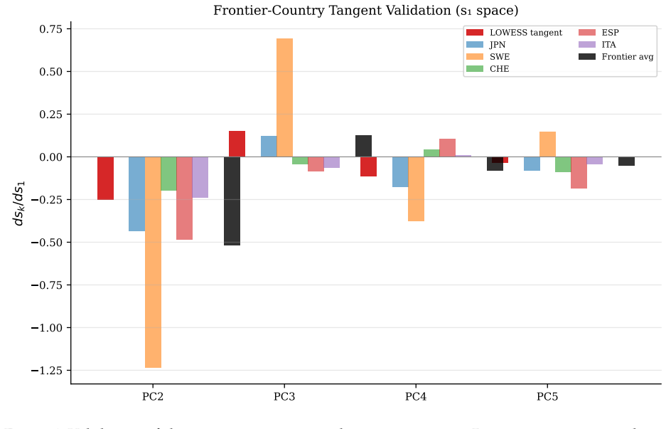
- [PCA reduction of Tucker score space] Section describing the PCA step on Tucker scores: the claim that the mortality transition is 'essentially one-dimensional' is not supported by any reported eigenvalues, scree plot, or cumulative variance percentages. Without these quantities it is impossible to judge whether the first principal component captures the large majority of variation or whether higher-order components encode independent structural shifts (e.g., infant versus senescence patterns) that a scalar speed function cannot reproduce at 50-year horizons.
- [Leave-country-out cross-validation] Cross-validation section: the leave-country-out procedure must specify exactly how the speed function and trajectory functions are estimated from training countries only, and what data-exclusion rules are applied to avoid leakage when the held-out countries' schedules are reconstructed. The current description leaves open the possibility that the reported bias and error reductions partly reflect in-sample structure rather than genuine out-of-sample forecasting skill.
- [Flow-field construction and integration] Flow-field integration description: the scalar speed function is fitted on historical data; the manuscript does not demonstrate that this function remains valid when extrapolated to horizons beyond the training window, nor does it provide sensitivity checks on the integration step when the speed function is perturbed within its estimation uncertainty.
minor comments (2)
- [Abstract] The abstract refers to 'our de novo Python reimplementation of the UN pipeline' but the main text does not indicate whether the code or the exact parameter settings used for that baseline are supplied as supplementary material.
- [Notation and definitions] Notation for the Tucker core tensor and the subsequent PCA loadings should be introduced once and used consistently; occasional switches between score-space and original-age-space symbols reduce readability.
Simulated Author's Rebuttal
We thank the referee for the constructive and detailed comments, which highlight important areas for clarification and strengthening of the manuscript. We address each major comment below, indicating the revisions we will make.
read point-by-point responses
-
Referee: Section describing the PCA step on Tucker scores: the claim that the mortality transition is 'essentially one-dimensional' is not supported by any reported eigenvalues, scree plot, or cumulative variance percentages. Without these quantities it is impossible to judge whether the first principal component captures the large majority of variation or whether higher-order components encode independent structural shifts (e.g., infant versus senescence patterns) that a scalar speed function cannot reproduce at 50-year horizons.
Authors: We agree that the manuscript should provide quantitative support for the one-dimensional claim. In the revised version, we will add the eigenvalues of the PCA applied to the Tucker scores, a scree plot, and the cumulative variance percentages. These additions will allow readers to evaluate the dominance of the first principal component and assess whether higher-order components capture independent structural shifts that might require more than a scalar speed function. revision: yes
-
Referee: Cross-validation section: the leave-country-out procedure must specify exactly how the speed function and trajectory functions are estimated from training countries only, and what data-exclusion rules are applied to avoid leakage when the held-out countries' schedules are reconstructed. The current description leaves open the possibility that the reported bias and error reductions partly reflect in-sample structure rather than genuine out-of-sample forecasting skill.
Authors: We will revise the cross-validation section to provide a precise, step-by-step description of the procedure. The Tucker decomposition will be performed solely on the training countries, and both the speed function and trajectory functions will be estimated exclusively from those training data. Held-out countries will be used only for evaluation, with explicit data-exclusion rules to prevent any leakage. This clarification will confirm the out-of-sample nature of the reported results. revision: yes
-
Referee: Flow-field integration description: the scalar speed function is fitted on historical data; the manuscript does not demonstrate that this function remains valid when extrapolated to horizons beyond the training window, nor does it provide sensitivity checks on the integration step when the speed function is perturbed within its estimation uncertainty.
Authors: The flow-field approach keeps forecasts within the empirically observed score manifold, which inherently limits extrapolation outside the range of historical dynamics. Nevertheless, we acknowledge the value of explicit sensitivity analysis. In the revision, we will add checks that perturb the speed function within its estimation uncertainty (e.g., via bootstrap resampling) and report the resulting variation in long-horizon forecasts, thereby demonstrating robustness. revision: partial
Circularity Check
No significant circularity in derivation chain
full rationale
The paper's core derivation applies Tucker decomposition to the Human Mortality Database, performs PCA on the resulting scores to identify a one-dimensional structure, and constructs a flow-field model with scalar speed and trajectory functions for forecasting. This structure is discovered from training data and then used to generate out-of-sample forecasts. Performance is assessed via leave-country-out cross-validation on 9,507 held-out test points from separate countries, providing independent evaluation. No quoted step reduces the forecasting mechanism or reported metrics to the inputs by construction, self-definition, or self-citation load-bearing; the model is a data-driven parameterization evaluated externally to its fitting data.
Axiom & Free-Parameter Ledger
free parameters (2)
- scalar speed function
- trajectory functions
axioms (1)
- domain assumption The mortality transition is essentially a one-dimensional flow in the low-dimensional Tucker score space.
invented entities (1)
-
flow field
no independent evidence
Lean theorems connected to this paper
-
IndisputableMonolith/Foundation/RealityFromDistinction.leanreality_from_one_distinction unclear?
unclearRelation between the paper passage and the cited Recognition theorem.
PCA reduction reveals that the mortality transition is essentially a one-dimensional flow: a scalar speed function advances the level, trajectory functions supply the structural scores
-
IndisputableMonolith/Cost/FunctionalEquation.leanwashburn_uniqueness_aczel unclear?
unclearRelation between the paper passage and the cited Recognition theorem.
speed function g*(s1) = ds1/dt estimated by LOWESS regression
What do these tags mean?
- matches
- The paper's claim is directly supported by a theorem in the formal canon.
- supports
- The theorem supports part of the paper's argument, but the paper may add assumptions or extra steps.
- extends
- The paper goes beyond the formal theorem; the theorem is a base layer rather than the whole result.
- uses
- The paper appears to rely on the theorem as machinery.
- contradicts
- The paper's claim conflicts with a theorem or certificate in the canon.
- unclear
- Pith found a possible connection, but the passage is too broad, indirect, or ambiguous to say the theorem truly supports the claim.
Reference graph
Works this paper leans on
-
[1]
doi:10.1126/science.aat3119. U. Basellini, C. G. Camarda, and H. Booth. Thirty years on: A review of the Lee–Carter method for forecasting mortality.International Journal of Forecasting, 39(3):1033–1049,
-
[2]
doi:10.1016/j.ijforecast.2022.11.002. M. Betancourt. A conceptual introduction to Hamiltonian Monte Carlo.arXiv preprint,
-
[3]
A Conceptual Introduction to Hamiltonian Monte Carlo
doi:10.48550/arXiv.1701.02434. URLhttps://arxiv.org/abs/1701.02434. H. Booth and L. Tickle. Mortality modelling and forecasting: A review of methods.Annals of Actuarial Science, 3(1–2):3–43,
work page internal anchor Pith review Pith/arXiv arXiv doi:10.48550/arxiv.1701.02434
-
[4]
doi:10.1017/S1748499500000440. H. Booth, L. Tickle, and L. Smith. Evaluation of the variants of the Lee–Carter method of forecasting mortality: A multicountry comparison.New Zealand Population Review, 31–32:13–34,
-
[5]
doi:10.1007/s13524-019- 00785-3. S. J. Clark. Multi-dimensional mortality with exceptional mortality from armed conflict and pandemics (MDMx). arXiv preprint arXiv:2603.20518,
-
[6]
doi:10.1080/08898480500452109. X. Dong, B. Milholland, and J. Vijg. Evidence for a limit to human lifespan.Nature, 538(7624): 257–259,
-
[7]
doi:10.1038/nature19793. Y. Dong, F. Huang, and S. Haberman. Multi-population mortality forecasting using tensor decompo- sition.Scandinavian Actuarial Journal, 2020(8):754–775,
-
[8]
doi:10.1080/03461238.2020.1740314. J. F. Fries. Aging, natural death, and the compression of morbidity.New England Journal of Medicine, 303(3):130–135,
-
[9]
doi:10.1056/NEJM198007173030304. M. D. Hoffman and A. Gelman. The No-U-Turn sampler: Adaptively setting path lengths in Hamiltonian Monte Carlo.Journal of Machine Learning Research, 15(47):1593–1623,
-
[10]
doi:10.1016/j.csda.2006.07.028. R. J. Hyndman, H. Booth, and F. Yasmeen. Coherent mortality forecasting: The product-ratio method with functional time series models.Demography, 50(1):261–283,
-
[11]
doi:10.1007/s13524- 012-0145-5. V . Kannisto.Development of Oldest-Old Mortality, 1950–1990: Evidence from 28 Developed Countries, volume 1 ofOdense Monographs on Population Aging. Odense University Press, Odense,
-
[12]
doi:10.1353/dem.2001.0036. R. D. Lee and L. R. Carter. Modeling and forecasting U.S. mortality.Journal of the American Statistical Association, 87(419):659–671,
-
[13]
doi:10.1080/01621459.1992.10475265. N. Li and R. Lee. Coherent mortality forecasts for a group of populations: An extension of the Lee–Carter method.Demography, 42(3):575–594,
-
[14]
doi:10.1353/dem.2005.0021. N. Li, R. Lee, and P . Gerland. Extending the Lee–Carter method to model the rotation of age patterns of mortality decline for long-term projections.Demography, 50(6):2037–2051,
-
[15]
doi:10.1007/s13524-013-0232-2. J. Oeppen and J. W. Vaupel. Broken limits to life expectancy.Science, 296(5570):1029–1031,
-
[16]
doi:10.1126/science.1069675. S. J. Olshansky, B. A. Carnes, and C. Cassel. In search of Methuselah: Estimating the upper limits to human longevity.Science, 250(4981):634–640,
-
[17]
doi:10.1126/science.2237414. S. J. Olshansky, B. J. Willcox, L. Demetrius, and H. Beltrán-Sánchez. Implausibility of radical life extension in humans in the twenty-first century.Nature Aging, 4(11):1635–1642,
-
[18]
doi:10.1038/s43587-024-00702-3. O. Papaspiliopoulos, G. O. Roberts, and M. Sköld. A general framework for the parametrization of hierarchical models.Statistical Science, 22(1):59–73,
-
[19]
doi:10.1214/088342307000000014. D. Phan, N. Pradhan, and M. Jankowiak. Composable effects for flexible and accelerated probabilis- tic programming in NumPyro. InAdvances in Neural Information Processing Systems,
-
[20]
doi:10.1007/s13524-012-0193-x. A. E. Raftery, N. Lali´ c, and P . Gerland. Joint probabilistic projection of female and male life expectancy.Demographic Research, 30:795–822,
-
[21]
doi:10.4054/DemRes.2014.30.27. M. Russolillo, G. Giordano, and S. Haberman. Extending the Lee–Carter model: A three-way decom- position.Scandinavian Actuarial Journal, 2011(2):96–117,
-
[22]
doi:10.1080/03461231003611933. H. Ševˇ cíková and A. E. Raftery.bayesLife: Bayesian Projection of Life Expectancy,
-
[23]
doi:10.1007/978-3-319-26603-9_15. H. Ševˇ cíková, L. Alkema, and A. E. Raftery.bayesTFR: Bayesian Fertility Projection, 2024a. URL https://CRAN.R-project.org/package=bayesTFR. R package version 7.4-4. H. Ševˇ cíková, N. Li, and P . Gerland.MortCast: Estimation and Projection of Age-Specific Mortality Rates, 2024b. URLhttps://CRAN.R-project.org/package=Mor...
-
[24]
doi:10.1038/nature08984. X. Zhang, F. Huang, F. K. C. Hui, and S. Haberman. Cause-of-death mortality forecasting using adaptive penalized tensor decompositions.Insurance: Mathematics and Economics, 111:193–213,
-
[25]
doi:10.1016/j.insmatheco.2023.05.003. 68
discussion (0)
Sign in with ORCID, Apple, or X to comment. Anyone can read and Pith papers without signing in.