Recognition: no theorem link
Scientific Validation of the SPARC4 Pipeline: Multi-band Imaging, Polarimetry, and Photometric Time Series for Improved Characterization of Transiting Exoplanets
Pith reviewed 2026-05-10 19:55 UTC · model grok-4.3
The pith
SPARC4 pipeline delivers 0.02% photometric precision on exoplanet transits and refines parameters via joint TESS modeling.
A machine-rendered reading of the paper's core claim, the machinery that carries it, and where it could break.
Core claim
The SPARC4 Pipeline processes high-cadence multi-band imaging and polarimetry to generate time series that achieve 0.02% photometric precision for a 15-minute cadence and 0.02% polarimetric precision over hours-long observations; joint Bayesian MCMC modeling of these light curves with TESS (or K2) data then produces refined constraints on the orbital periods and radii of the observed hot Jupiters.
What carries the argument
The SPARC4 Pipeline, a suite of routines that calibrates images, extracts time series, and feeds them into Bayesian MCMC joint modeling with space-based photometry.
If this is right
- Orbital periods and planetary radii for the observed hot Jupiters can be determined more accurately than with either dataset alone.
- Multi-band and polarimetric time series become practical for ground-based characterization of transiting planets with host stars of V = 10 to 14.
- The same reduction steps can be applied to other exoplanet systems observed with SPARC4 to produce comparable photometric and polarimetric time series.
- Instrumental polarization remains below 0.06%, enabling reliable linear polarization measurements at the 0.2% level for future programs.
Where Pith is reading between the lines
- The demonstrated precision level suggests SPARC4 could contribute to ground-based follow-up of TESS discoveries that require multi-band or polarimetric information.
- Joint modeling approaches of this type may become standard for combining ground-based high-cadence data with space photometry to reduce parameter degeneracies.
- If the pipeline performance holds across a wider range of targets and conditions, similar instrument-specific pipelines could be developed for other small telescopes.
Load-bearing premise
The pipeline fully removes instrumental systematics and the seven chosen transits plus standard-star observations are representative enough to support the quoted precision and improved parameter constraints.
What would settle it
A new transit observation of one of the same systems with an independent high-precision instrument that yields a planetary radius differing by more than the reported uncertainty from the joint SPARC4-plus-TESS value.
Figures


read the original abstract
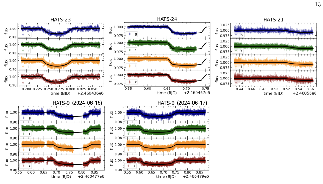
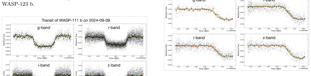
High-cadence multi-band imaging and polarimetry have important scientific applications in astronomy. Observations of transits of exoplanets are a particular application that requires robust data reduction and analysis. We present the SPARC4 Pipeline, a suite of routines developed to process photometric and polarimetric data obtained with the instrument SPARC4 installed on the 1.6 m telescope at Pico dos Dias Observatory, Brazil. The scientific data products, up to the generation of high-cadence time series, are demonstrated using observations of several transiting exoplanetary systems in both photometric and polarimetric modes. These observations are used to produce stacked calibrated images, yielding sub-arcsecond astrometric accuracy even in sparse fields. The time series of these fields enabled a photometric characterization of the instrument. Observations of polarimetric standard stars yield an instrumental polarization below 0.06% and a linear polarization accuracy of 0.2%. Furthermore, transit observations of seven exoplanets with host-star magnitudes in the range 10.2 < V < 13.9 demonstrate that SPARC4 achieves an average photometric precision of 0.02% for a 15-minute cadence and a polarimetric precision of ~0.02% over hours-long time series. Finally, we jointly model the SPARC4 light curves together with TESS data (or K2 data in the case of HATS-9) using a Bayesian MCMC framework to refine constraints on the physical parameters of the exoplanets, enabling a more accurate determination of orbital periods and planetary radii, and providing improved constraints on the orbital and physical parameters of these hot Jupiters.
Editorial analysis
A structured set of objections, weighed in public.
Referee Report
Summary. The manuscript introduces the SPARC4 Pipeline for reducing multi-band imaging and polarimetric data acquired with the SPARC4 instrument on the 1.6 m telescope at Pico dos Dias Observatory. It validates the pipeline through observations of polarimetric standard stars (yielding instrumental polarization below 0.06% and linear polarization accuracy of 0.2%) and seven transiting exoplanets (host magnitudes 10.2 < V < 13.9), reporting an average photometric precision of 0.02% at 15-minute cadence and polarimetric precision of ~0.02% over hours-long time series. The work further demonstrates that joint Bayesian MCMC modeling of the SPARC4 light curves with TESS (or K2) photometry refines constraints on orbital periods, planetary radii, and other physical parameters of the hot Jupiters.
Significance. If the reported precisions and improvements hold, the paper is significant for delivering a validated, publicly usable pipeline that enables competitive ground-based high-cadence photometry and polarimetry, directly supporting exoplanet characterization. The joint-modeling results illustrate a practical route for combining ground-based multi-band data with space photometry to tighten parameter posteriors. The manuscript addresses the representativeness concern by supplying per-target light-curve figures, residual-noise analysis, and before/after parameter tables, so the weakest assumption in the stress-test note does not materialize as a load-bearing gap.
minor comments (2)
- Abstract: the phrase 'sub-arcsecond astrometric accuracy' is stated without a quantitative example or table entry; adding a short table or sentence with measured RMS values across the seven fields would strengthen the claim.
- Results section: the 15-minute cadence used for the 0.02% photometric precision metric should be defined explicitly (e.g., bin size, number of points per bin) to allow direct comparison with other instruments.
Simulated Author's Rebuttal
We thank the referee for the positive assessment of the SPARC4 pipeline manuscript and the recommendation for minor revision. No specific major comments were raised in the report.
Circularity Check
No significant circularity in derivation chain
full rationale
The paper validates the SPARC4 pipeline through direct empirical measurements of instrumental polarization and photometric precision on standard stars and seven transit observations, then applies standard Bayesian MCMC joint modeling with independent external TESS/K2 datasets. No load-bearing equations, fitted parameters renamed as predictions, or self-citation chains reduce the reported precisions or refined exoplanet parameters to quantities defined solely by the authors' own inputs or prior assumptions. The central claims rest on observable data products and external benchmarks without self-referential reduction.
Axiom & Free-Parameter Ledger
axioms (1)
- domain assumption Standard assumptions in exoplanet transit modeling hold, including appropriate limb-darkening laws and negligible unmodeled stellar activity in the chosen targets.
Reference graph
Works this paper leans on
-
[1]
Adibekyan, V., Dorn, C., Sousa, S. G., et al. 2021, Science, 374, 330, doi: 10.1126/science.abg8794
-
[2]
Anderson, D. R., Brown, D. J. A., Collier Cameron, A., et al. 2014, arXiv e-prints, arXiv:1410.3449, doi: 10.48550/arXiv.1410.3449 Astropy Collaboration, Robitaille, T. P., Tollerud, E. J., et al. 2013, A&A, 558, A33, doi: 10.1051/0004-6361/201322068 Astropy Collaboration, Price-Whelan, A. M., Sip˝ ocz, B. M., et al. 2018, AJ, 156, 123, doi: 10.3847/1538-...
-
[3]
Bento, J., Schmidt, B., Hartman, J. D., et al. 2017, MNRAS, 468, 835, doi: 10.1093/mnras/stx500
-
[4]
2025, PhD thesis, Brazilian National Institute for Space Research
Bernardes, D. 2025, PhD thesis, Brazilian National Institute for Space Research
2025
-
[5]
Bernardes, D., Junior, O. V., Rodrigues, F., et al. 2025, PASP, 137, 035003, doi: 10.1088/1538-3873/ada187
-
[6]
Beroiz, M., Cabral, J. B., & Sanchez, B. 2020, Astronomy and Computing, 32, 100384, doi: 10.1016/j.ascom.2020.100384
-
[7]
Bhatti, W., Bakos, G. ´A., Hartman, J. D., et al. 2016, arXiv e-prints, arXiv:1607.00322, doi: 10.48550/arXiv.1607.00322
-
[8]
2024, astropy/photutils: 2.0.2, 2.0.2, Zenodo, doi: 10.5281/zenodo.13989456
Bradley, L., Sip˝ ocz, B., Robitaille, T., et al. 2024, astropy/photutils: 2.0.2, 2.0.2, Zenodo, doi: 10.5281/zenodo.13989456
-
[9]
Brahm, R., Jord´ an, A., Hartman, J. D., et al. 2015, AJ, 150, 33, doi: 10.1088/0004-6256/150/1/33
-
[10]
Calabretta, M. R., & Greisen, E. W. 2002, A&A, 395, 1077, doi: 10.1051/0004-6361:20021327
-
[11]
Campagnolo, J. C. N. 2018, ASTROPOP: ASTROnomical Polarimetry and Photometry pipeline, Astrophysics Source Code Library, record ascl:1805.024
2018
-
[12]
Carciofi, A. C., & Magalh˜ aes, A. M. 2005, ApJ, 635, 570, doi: 10.1086/497064
-
[13]
2017, MNRAS, 464, 4146, doi: 10.1093/mnras/stw2545
Cikota, A., Patat, F., Cikota, S., & Faran, T. 2017, MNRAS, 464, 4146, doi: 10.1093/mnras/stw2545
-
[14]
2017, A&A, 600, A30, doi: 10.1051/0004-6361/201629705
Claret, A. 2017, A&A, 600, A30, doi: 10.1051/0004-6361/201629705
-
[15]
Claret, A., & Bloemen, S. 2011, A&A, 529, A75, doi: 10.1051/0004-6361/201116451
-
[16]
2019, PASP, 131, 013001, doi: 10.1088/1538-3873/aae5c5
Deming, D., Louie, D., & Sheets, H. 2019, PASP, 131, 013001, doi: 10.1088/1538-3873/aae5c5
-
[17]
Dorn, C., Khan, A., Heng, K., et al. 2015, A&A, 577, A83, doi: 10.1051/0004-6361/201424915
-
[18]
Foreman-Mackey, D., Hogg, D. W., Lang, D., & Goodman, J. 2013, PASP, 125, 306, doi: 10.1086/670067 30 Figure 16.TESS (or K2) light curves of the seven exoplanet transits analyzed in this work. Light blue points show the photometric data around the transits, dark blue points show binned data (bin size 0.002 d), and red lines indicate the best-fit joint SPA...
-
[19]
2007, in Astronomical Society of the Pacific Conference Series, Vol
Fossati, L., Bagnulo, S., Mason, E., & Landi Degl’Innocenti, E. 2007, in Astronomical Society of the Pacific Conference Series, Vol. 364, The Future of
2007
-
[20]
Fukugita, M., Ichikawa, T., Gunn, J. E., et al. 1996, AJ, 111, 1748, doi: 10.1086/117915
-
[21]
Ginsburg, A., Sip˝ ocz, B. M., Brasseur, C. E., et al. 2019, AJ, 157, 98, doi: 10.3847/1538-3881/aafc33
-
[22]
Greisen, E. W., & Calabretta, M. R. 2002, A&A, 395, 1061, doi: 10.1051/0004-6361:20021326
-
[23]
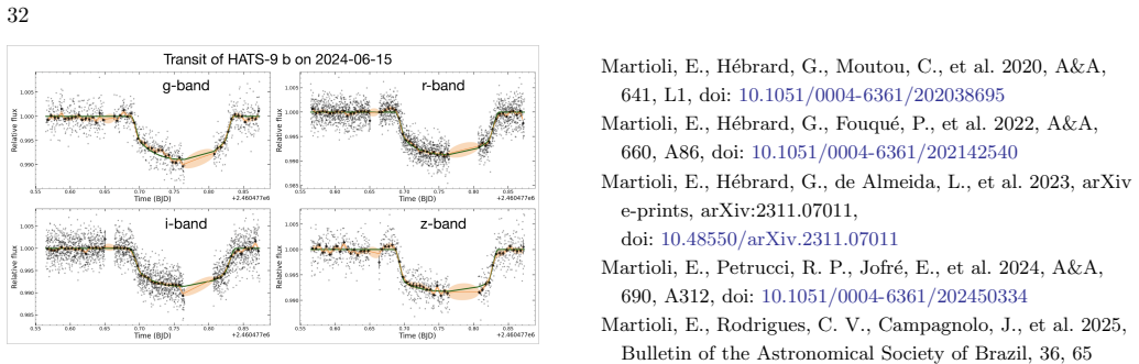
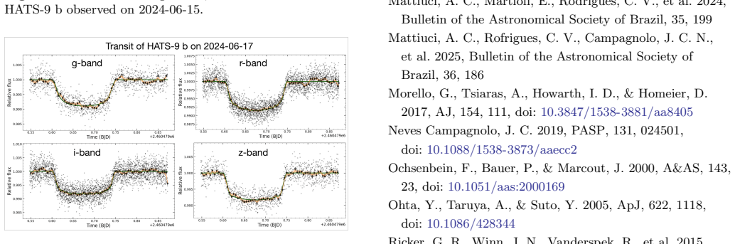
Harris, W. E., Fitzgerald, M. P., & Reed, B. C. 1981, PASP, 93, 507, doi: 10.1086/130868 32 Figure 23.Same as Figure 17, but for the transit of HATS-9 b observed on 2024-06-15. Figure 24.Same as Figure 17, but for the transit of HATS-9 b observed on 2024-06-17
-
[24]
B., Sobeck, C., Haas, M., et al
Howell, S. B., Sobeck, C., Haas, M., et al. 2014, PASP, 126, 398, doi: 10.1086/676406
-
[25]
Hunter, J. D. 2007, Computing in Science and Engineering, 9, 90, doi: 10.1109/MCSE.2007.55
-
[26]
1994, PASP, 106, 1172, doi: 10.1086/133495
Jablonski, F., Baptista, R., Barroso, J., et al. 1994, PASP, 106, 1172, doi: 10.1086/133495
-
[27]
Kostogryz, N. M., Yakobchuk, T. M., & Berdyugina, S. V. 2015, ApJ, 806, 97, doi: 10.1088/0004-637X/806/1/97
-
[28]
2015, Publications of the Astronomical Society of the Pacific, 127, 1161, doi: 10.1086/683602
Kreidberg, L. 2015, PASP, 127, 1161, doi: 10.1086/683602 Lightkurve Collaboration, Cardoso, J. V. d. M., Hedges, C., et al. 2018, Lightkurve: Kepler and TESS time series analysis in Python, Astrophysics Source Code Library. http://ascl.net/1812.013
-
[29]
Lima, I. J., Rodrigues, C. V., Ferreira Lopes, C. E., et al. 2021, AJ, 161, 225, doi: 10.3847/1538-3881/abeb16 Magalh˜ aes, A. M., Benedetti, E., & Roland, E. H. 1984, PASP, 96, 383, doi: 10.1086/131351
-
[30]
Martioli, E., H´ ebrard, G., Correia, A. C. M., Laskar, J., & Lecavelier des Etangs, A. 2021, A&A, 649, A177, doi: 10.1051/0004-6361/202040235
-
[31]
Martioli, E., Col´ on, K. D., Angerhausen, D., et al. 2018, MNRAS, 474, 4264, doi: 10.1093/mnras/stx3009
-
[32]
2020, A&A, 641, L1, doi: 10.1051/0004-6361/202038695
Martioli, E., H´ ebrard, G., Moutou, C., et al. 2020, A&A, 641, L1, doi: 10.1051/0004-6361/202038695
-
[33]
2022, A&A, 660, A86, doi: 10.1051/0004-6361/202142540
Martioli, E., H´ ebrard, G., Fouqu´ e, P., et al. 2022, A&A, 660, A86, doi: 10.1051/0004-6361/202142540
-
[34]
2023, arXiv e-prints, arXiv:2311.07011, doi: 10.48550/arXiv.2311.07011
Martioli, E., H´ ebrard, G., de Almeida, L., et al. 2023, arXiv e-prints, arXiv:2311.07011, doi: 10.48550/arXiv.2311.07011
-
[35]
Martioli, E., Petrucci, R. P., Jofr´ e, E., et al. 2024, A&A, 690, A312, doi: 10.1051/0004-6361/202450334
-
[36]
V., Campagnolo, J., et al
Martioli, E., Rodrigues, C. V., Campagnolo, J., et al. 2025, Bulletin of the Astronomical Society of Brazil, 36, 65
2025
-
[37]
C., Martioli, E., Rodrigues, C
Mattiuci, A. C., Martioli, E., Rodrigues, C. V., et al. 2024, Bulletin of the Astronomical Society of Brazil, 35, 199
2024
-
[38]
C., Rofrigues, C
Mattiuci, A. C., Rofrigues, C. V., Campagnolo, J. C. N., et al. 2025, Bulletin of the Astronomical Society of Brazil, 36, 186
2025
-
[39]
Morello, G., Tsiaras, A., Howarth, I. D., & Homeier, D. 2017, AJ, 154, 111, doi: 10.3847/1538-3881/aa8405 Neves Campagnolo, J. C. 2019, PASP, 131, 024501, doi: 10.1088/1538-3873/aaecc2
-
[40]
Astronomy and Astrophysics Supplement Series , author =
Ochsenbein, F., Bauer, P., & Marcout, J. 2000, A&AS, 143, 23, doi: 10.1051/aas:2000169
-
[41]
2005, ApJ, 622, 1118, doi: 10.1086/428344
Ohta, Y., Taruya, A., & Suto, Y. 2005, ApJ, 622, 1118, doi: 10.1086/428344
-
[42]
doi:10.1117/1.JATIS.1.1.014003 , eid =
Ricker, G. R., Winn, J. N., Vanderspek, R., et al. 2015, Journal of Astronomical Telescopes, Instruments, and Systems, 1, 014003, doi: 10.1117/1.JATIS.1.1.014003
work page internal anchor Pith review doi:10.1117/1.jatis.1.1.014003 2015
-
[43]
V., Cieslinski, D., & Steiner, J
Rodrigues, C. V., Cieslinski, D., & Steiner, J. E. 1998, A&A, 335, 979, doi: 10.48550/arXiv.astro-ph/9805193
work page internal anchor Pith review doi:10.48550/arxiv.astro-ph/9805193 1998
-
[44]
V., Taylor, K., Jablonski, F
Rodrigues, C. V., Taylor, K., Jablonski, F. J., et al. 2012, in Society of Photo-Optical Instrumentation Engineers (SPIE) Conference Series, Vol. 8446, Ground-based and Airborne Instrumentation for Astronomy IV, ed. I. S
2012
-
[45]
McLean, S. K. Ramsay, & H. Takami, 844626, doi: 10.1117/12.924976
-
[46]
V., Gneiding, C
Rodrigues, C. V., Gneiding, C. D., Almeida, L., et al. 2024, Bulletin of the Astronomical Society of Brazil, 35, 44
2024
-
[47]
Schlindwein, W., Campagnolo, J. C. N., Martioli, E., et al. 2024, Bulletin of the Astronomical Society of Brazil, 35, 313
2024
-
[48]
2010, Exoplanet Atmospheres: Physical Processes
Seager, S. 2010, Exoplanet Atmospheres: Physical Processes
2010
-
[49]
Serkowski, K., Mathewson, D. S., & Ford, V. L. 1975, ApJ, 196, 261, doi: 10.1086/153410
-
[50]
R., Collier-Cameron, A., et al
Smalley, B., Anderson, D. R., Collier-Cameron, A., et al. 2012, A&A, 547, A61, doi: 10.1051/0004-6361/201219731
-
[51]
Snellen, I. A. G., & Brown, A. G. A. 2018, Nature Astronomy, 2, 883, doi: 10.1038/s41550-018-0561-6
-
[52]
Turner, O. D., Anderson, D. R., Collier Cameron, A., et al. 2016, PASP, 128, 064401, doi: 10.1088/1538-3873/128/964/064401 33
-
[53]
Valio, A., Martioli, E., Kovacs, A. O., et al. 2025, arXiv e-prints, arXiv:2510.08424. https://arxiv.org/abs/2510.08424 Van Der Walt, S., Colbert, S. C., & Varoquaux, G. 2011, Computing in Science and Engineering, 13, 22, doi: 10.1109/MCSE.2011.37
-
[54]
2000, , 143, 9, 10.1051/aas:2000332
Wenger, M., Ochsenbein, F., Egret, D., et al. 2000, A&AS, 143, 9, doi: 10.1051/aas:2000332
work page internal anchor Pith review doi:10.1051/aas:2000332 2000
-
[55]
Wolf, C., Onken, C. A., Luvaul, L. C., et al. 2018, PASA, 35, e010, doi: 10.1017/pasa.2018.5
discussion (0)
Sign in with ORCID, Apple, or X to comment. Anyone can read and Pith papers without signing in.