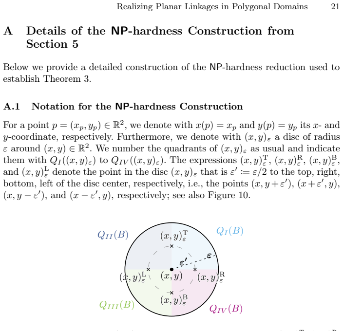
Recognition: no theorem link
Realizing Planar Linkages in Polygonal Domains
Pith reviewed 2026-05-10 18:31 UTC · model grok-4.3
The pith
Realizing a linkage inside a polygonal domain is W[1]-hard in the number of vertices even for unit lengths and no prescribed positions.
A machine-rendered reading of the paper's core claim, the machinery that carries it, and where it could break.
Core claim
We show XP-membership and W[1]-hardness with respect to the size of G, even if ℓ ≡ 1 and no vertex positions are prescribed. Furthermore, we consider the case where G is a path with prescribed start and end position and ℓ ≡ 1. Despite the absence of any rigid components, we obtain NP-hardness in general, and provide a linear-time algorithm for arbitrary ℓ if G has only three edges and P is convex.
What carries the argument
The linkage realization problem inside an open polygonal domain P, which uses the interior geometry of P to enforce global planarity and length constraints while allowing reductions that encode combinatorial hardness.
If this is right
- The hardness persists for completely flexible linkages that contain no rigid subgraphs.
- Prescribing only the two endpoints of a path is already enough to make the realization question NP-hard inside general polygons.
- Convexity of the domain together with a constant number of edges restores linear-time solvability even for arbitrary edge lengths.
- The results separate the source of hardness from rigidity: the interaction between the linkage and the domain boundary suffices.
Where Pith is reading between the lines
- Similar parameterized hardness may hold when the domain is required to be simply connected or when a small number of interior obstacles are added.
- It would be natural to ask whether the three-edge linear-time result extends to a constant number of edges inside polygons of bounded complexity.
- The same geometric encoding technique might yield hardness for approximate realization or for maximizing the number of vertices that fit inside a fixed domain.
Load-bearing premise
The domain P must be open and every valid realization must lie strictly inside P without touching the boundary, so that reductions can place vertices and edges to simulate choices without violating planarity or escaping the region.
What would settle it
An algorithm that, for any fixed number of vertices, decides in polynomial time whether a unit-length linkage realizes inside a given polygonal domain, or an explicit small instance with five vertices where no such realization exists despite satisfying all local length and non-crossing conditions.
Figures


read the original abstract
A linkage $\mathcal{L}$ consists of a graph $G=(V,E)$ and an edge-length function $\ell$. Deciding whether $\mathcal{L}$ can be realized as a planar straight-line embedding in $\mathbb{R}^2$ with edge length $\ell(e)$ for all $e \in E$ is $\exists\mathbb{R}$-complete [Abel et al., JoCG'25], even if $\ell \equiv 1$, but a considerable part of $\mathcal{L}$ is rigid. In this paper, we study the computational complexity of the realization question for structurally simpler, less rigid linkages inside an open polygonal domain $P$, where the placement of some vertices may be specified in the input. We show XP-membership and W[1]-hardness with respect to the size of $G$, even if $\ell \equiv 1$ and no vertex positions are prescribed. Furthermore, we consider the case where $G$ is a path with prescribed start and end position and $\ell \equiv 1$. Despite the absence of any rigid components, we obtain NP-hardness in general, and provide a linear-time algorithm for arbitrary $\ell$ if $G$ has only three edges and $P$ is convex.
Editorial analysis
A structured set of objections, weighed in public.
Referee Report
Summary. The manuscript studies the computational complexity of realizing a linkage (a graph G with edge lengths ℓ) as a planar straight-line embedding strictly inside an open polygonal domain P, where some vertices may have prescribed positions. It establishes XP-membership and W[1]-hardness parameterized by |V(G)|, even when ℓ ≡ 1 and no positions are fixed. For the special case of path linkages with fixed endpoints and unit lengths, it proves NP-hardness in general via a 3-SAT reduction, while providing a linear-time algorithm when |E| = 3 and P is convex.
Significance. If the results hold, this work meaningfully refines the complexity map for linkage realization by isolating the effects of domain constraints and reduced rigidity. The explicit XP algorithm via bounded enumeration of vertex-order types inside P, the W[1]-hardness reduction using unit-length gadgets along the boundary, and the linear-time sweep for the three-edge convex case are concrete strengths that provide both negative and positive results without relying on rigid substructures.
minor comments (2)
- [§3] §3 (XP membership): the enumeration of order types is described at a high level; adding a brief pseudocode sketch or a small worked example would improve readability without altering the argument.
- [§5] The statement of the linear-time algorithm for |E|=3 (convex P) would benefit from an explicit statement of the running-time constant or the sweep primitives used, to make the O(n) claim fully transparent.
Simulated Author's Rebuttal
We thank the referee for their positive evaluation of the manuscript and for recommending minor revision. The summary accurately captures the main contributions: the XP-membership and W[1]-hardness results for general linkages (even with unit lengths and no fixed positions), the NP-hardness for unit-length paths with fixed endpoints, and the linear-time algorithm for three-edge paths in convex polygons. We appreciate the recognition that these results help refine the complexity map without relying on rigid substructures.
Circularity Check
No significant circularity detected
full rationale
The paper's core results—XP-membership via bounded combinatorial enumeration of vertex-order types inside P, W[1]-hardness via a gadget reduction along the boundary, NP-hardness for paths via 3-SAT reduction staying strictly inside the open domain, and the linear-time algorithm for |E|=3 in convex P—are established through independent geometric reductions and direct algorithmic constructions. No step reduces by definition to its inputs, renames a known result, or relies on a load-bearing self-citation chain; the cited ∃R-completeness result is external and not used to derive the new claims.
Axiom & Free-Parameter Ledger
axioms (2)
- domain assumption Standard assumptions of parameterized complexity theory (FPT vs W[1]-hardness, XP membership)
- standard math NP-hardness reductions are valid when the target problem is in NP
Reference graph
Works this paper leans on
-
[1]
Abel, Z., Demaine, E.D., Demaine, M.L., Eisenstat, S., Lynch, J., Schardl, T.B.: Who Needs Crossings? Hardness of Plane Graph Rigidity. In: Fekete, S.P., Lu- biw, A. (eds.) Proc. 32nd International Symposium on Computational Geometry (SoCG’16). LIPIcs, vol. 51, pp. 3:1–3:15. Schloss Dagstuhl – Leibniz-Zentrum für Informatik (2016). https://doi.org/10.4230...
-
[2]
Journal of Computational Geometry16(2025)
Abel, Z., Demaine, E.D., Demaine, M.L., Eisenstat, S., Lynch, J., Schardl, T.B.: Who needs crossings?: Noncrossing linkages are universal, and deciding (global) rigidity is hard. Journal of Computational Geometry16(2025). https://doi.org/ 10.20382/JOCG.V16I1A12
-
[3]
TheoretiCS3(2024)
Abrahamsen, M., Miltzow, T., Seiferth, N.: Framework for∃∖-completeness of two-dimensional packing problems. TheoretiCS3(2024). https://doi.org/10. 46298/THEORETICS.24.11
2024
-
[4]
Alt, H., Knauer, C., Rote, G., Whitesides, S.: The complexity of (un)folding. In: Fortune, S. (ed.) Proc. 19th International Symposium on Computational Geometry (SoCG’03). pp. 164–170. ACM (2003). https://doi.org/10.1145/777792.777818 Realizing Planar Linkages in Polygonal Domains 19
-
[5]
In: Aichholzer, O., Wang, H
Angelini, P., Cornelsen, S., Haase, C., Hoffmann, M., Katsanou, E., Montecchi- ani, F., Steiner, R., Symvonis, A.: Geometric realizations of dichotomous ordi- nal graphs. In: Aichholzer, O., Wang, H. (eds.) Proc. 41st International Sym- posium on Computational Geometry (SoCG’25). LIPIcs, vol. 332, pp. 9:1–9:16. Schloss Dagstuhl – Leibniz-Zentrum für Infor...
2025
-
[6]
de Berg, M., Cheong, O., van Kreveld, M., Overmars, M.: Computational Geome- try: Algorithms and Applications (3rd Edition). Springer (2008). https://doi.org/ 10.1007/978-3-540-77974-2
-
[7]
International Journal of Computational Geometry and Application22(03), 187–205 (2012)
de Berg, M., Khosravi, A.: Optimal Binary Space Partitions for Segments in the Plane. International Journal of Computational Geometry and Application22(03), 187–205 (2012). https://doi.org/10.1142/s0218195912500045
-
[8]
Discrete Applied Mathematics117(1–3), 293–297 (2002)
Biedl, T., Demaine, E., Demaine, M., Lazard, S., Lubiw, A., O’Rourke, J., Robbins, S., Streinu, I., Toussaint, G., Whitesides, S.: A note on reconfiguring tree linkages: trees can lock. Discrete Applied Mathematics117(1–3), 293–297 (2002). https: //doi.org/10.1016/s0166-218x(01)00229-3
-
[9]
In: Liotta, G
Cabello, S., Demaine, E.D., Rote, G.: Planar Embeddings of Graphs with Spec- ified Edge Lengths. In: Liotta, G. (ed.) Proc. 11th International Symposium on Graph Drawing and Network Visualization (GD’03). LNCS, vol. 2912, pp. 283–
-
[10]
https://doi.org/10.1007/978-3-540-24595-7_26
Springer (2004). https://doi.org/10.1007/978-3-540-24595-7_26
-
[11]
Journal of Graph Algorithms and Applications11(1), 259–276 (2007)
Cabello, S., Demaine, E.D., Rote, G.: Planar Embeddings of Graphs with Speci- fied Edge Lengths. Journal of Graph Algorithms and Applications11(1), 259–276 (2007). https://doi.org/10.7155/jgaa.00145
-
[12]
Discrete & Computational Geometry30(2), 205–239 (2003)
Connelly, R., Demaine, E.D., Rote, G.: Straightening Polygonal Arcs and Con- vexifying Polygonal Cycles. Discrete & Computational Geometry30(2), 205–239 (2003). https://doi.org/10.1007/S00454-003-0006-7
-
[13]
Fomin and Lukasz Kowalik and Daniel Lokshtanov and D
Cygan, M., Fomin, F.V., Kowalik, L., Lokshtanov, D., Marx, D., Pilipczuk, M., Pilipczuk, M., Saurabh, S.: Parameterized Algorithms. Springer (2015). https:// doi.org/10.1007/978-3-319-21275-3
-
[14]
Cambridge University Press (2007)
Demaine, E.D., O’Rourke, J.: Geometric Folding Algorithms: Linkages, Origami, Polyhedra. Cambridge University Press (2007). https://doi.org/10.1017/ cbo9780511735172
2007
-
[15]
Dis- crete Applied Mathematics28(2), 111–134 (1990)
Eades, P., Wormald, N.C.: Fixed edge-length graph drawing is NP-hard. Dis- crete Applied Mathematics28(2), 111–134 (1990). https://doi.org/10.1016/ 0166-218x(90)90110-x
1990
-
[16]
SIAM Journal on Computing53(6), S20–102 (2024)
Erickson, J., van der Hoog, I., Miltzow, T.: Smoothing the gap between NP and ER. SIAM Journal on Computing53(6), S20–102 (2024). https://doi.org/10.1137/ 20M1385287
2024
-
[17]
Journal of Symbolic Computation5(1–2), 37–64 (1988)
Grigoriev, D., Jr., N.N.V.: Solving systems of polynomial inequalities in subex- ponential time. Journal of Symbolic Computation5(1–2), 37–64 (1988). https: //doi.org/10.1016/s0747-7171(88)80005-1
-
[18]
SIAM Journal on Computing13(3), 610–629 (1984)
Hopcroft, J., Joseph, D., Whitesides, S.: Movement Problems for 2-Dimensional Linkages. SIAM Journal on Computing13(3), 610–629 (1984). https://doi.org/10. 1137/0213038
1984
-
[19]
SIAM Journal on Computing14(2), 315–333 (1985)
Hopcroft, J., Joseph, D., Whitesides, S.: On the Movement of Robot Arms in 2-Dimensional Bounded Regions. SIAM Journal on Computing14(2), 315–333 (1985). https://doi.org/10.1137/0214025
-
[20]
Joseph, D.A., Plantings, W.H.: On the Complexity of Reachability and Motion Planning Questions (Extended Abstract). In: Proc. 1st International Symposium on Computational Geometry (SoCG). pp. 62–66. ACM (1985). https://doi.org/10. 1145/323233.323242 20 T. Depian, C. Haase, M. Nöllenburg, A. Schulz
-
[21]
Discrete & Com- putational Geometry7(1), 69–76 (1992)
Kantabutra, V.: Motions of a short-linked robot arm in a square. Discrete & Com- putational Geometry7(1), 69–76 (1992). https://doi.org/10.1007/bf02187825
-
[22]
Topology41(6), 1051–1107 (2002)
Kapovich, M., Millson, J.J.: Universality theorems for configuration spaces of planar linkages. Topology41(6), 1051–1107 (2002). https://doi.org/10.1016/ s0040-9383(01)00034-9
2002
-
[23]
Proceedings of the London Mathematical Society1(1), 213–216 (1875)
Kempe,A.B.:OnaGeneralMethodofdescribingPlaneCurvesofthenthdegreeby Linkwork. Proceedings of the London Mathematical Society1(1), 213–216 (1875). https://doi.org/10.1112/plms/s1-7.1.213
-
[24]
Lubiw, A., Miltzow, T., Mondal, D.: The complexity of drawing a graph in a polyg- onal region. In: Biedl, T., Kerren, A. (eds.) Proc. 26th International Symposium on Graph Drawing and Network Visualization (GD’18). pp. 387–401. Lecture Notes in Computer Science, Springer (2018). https://doi.org/10.1007/978-3-030-04414-5_ 28
-
[25]
Journal of Graph Algorithms and Applications26(4), 421–446 (2022)
Lubiw, A., Miltzow, T., Mondal, D.: The complexity of drawing a graph in a polygonal region. Journal of Graph Algorithms and Applications26(4), 421–446 (2022). https://doi.org/10.7155/jgaa.00602
-
[26]
Mitchell, J.S.B.: Geometric Shortest Paths and Network Optimization. In: Sack, J., Urrutia, J. (eds.) Handbook of Computational Geometry, chap. 15, pp. 633–701. Elsevier (2000). https://doi.org/10.1016/b978-044482537-7/50016-4
-
[27]
Preparata, F.P., Shamos, M.I.: Computational Geometry - An Introduction. Springer (1985). https://doi.org/10.1007/978-1-4612-1098-6
-
[28]
Whitesides, S., Pei, N.: On the Reconfiguration of Chains (Extended Abstract). In: Cai, J., Wong, C.K. (eds.) Proc. 2nd International Computing and Combinatorics Conference (COCOON’96). Lecture Notes in Computer Science, vol. 1090, pp. 381–390. Springer (1996). https://doi.org/10.1007/3-540-61332-3_172 Realizing Planar Linkages in Polygonal Domains 21 A D...
-
[29]
Towardsconstructingthesecondcorridor,(CC2),letc 1 bethe(unique)cross- ing of the two unit-disks positioned at(0,0.6)and(0,1)that lies insideB
We perform symmetrically forR2 1 and take the union ofR1 1 andR 2 1 without the “cut-off” from the triangles as (CC1). Towardsconstructingthesecondcorridor,(CC2),letc 1 bethe(unique)cross- ing of the two unit-disks positioned at(0,0.6)and(0,1)that lies insideB. Sim- ilarly, letc 2 be the (unique) crossing of the two unit-disks positioned at(0,1)R ε and(0,...
-
[30]
cut-away
To complete the construction of (CC5), we enlarge all rectangles such that they full-intersect at their ends Observe that (CC5) leans to the left and does not intersect (CC1). Corridor (CC6) is a symmetric (and mirrored) copy of (CC5) and it remains to construct (CC7). For the corridor (CC7), we takeR1 7, place its lower-left corner at(0.2,0)R ε and rotat...
-
[31]
From this on, Lemma 3 allows us to once more finalize the construction ofΓ ′ and we get Γ ′(vi+7)∈ → ¬xj (C)
To finalize the construction ofΓ ′, we observe thatΓ(v i+5) = (5,0)∈ → ¬xj (T2), for the second tunnelT 2 attached toC ′. From this on, Lemma 3 allows us to once more finalize the construction ofΓ ′ and we get Γ ′(vi+7)∈ → ¬xj (C). If the configuration should lean to the right, as in Figure 6b, we perform symmetrically. The last case withp∈ → y(C)can be h...
discussion (0)
Sign in with ORCID, Apple, or X to comment. Anyone can read and Pith papers without signing in.