Recognition: 2 theorem links
· Lean TheoremThe Transit Timing and Transmission Spectrum of Hot Jupiter WASP-43 b from a decade of Multi-band Transit Follow-up Observations
Pith reviewed 2026-05-10 18:54 UTC · model grok-4.3
The pith
Observations of hot Jupiter WASP-43 b over a decade show no significant orbital decay while revealing modeling difficulties when combining atmospheric spectra from multiple instruments.
A machine-rendered reading of the paper's core claim, the machinery that carries it, and where it could break.
Core claim
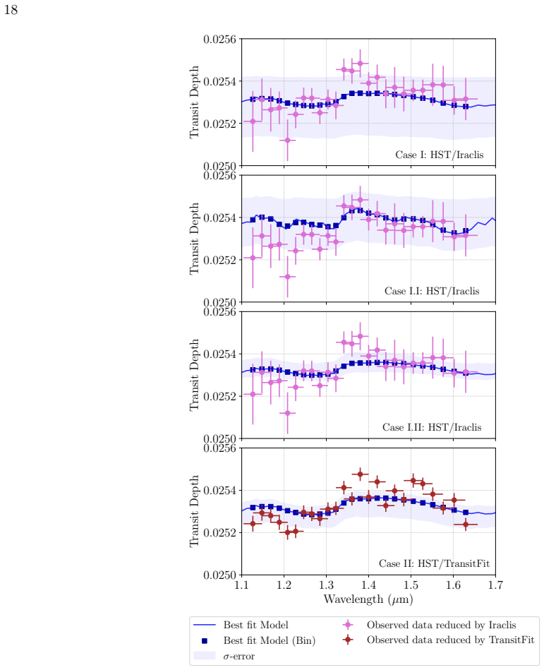
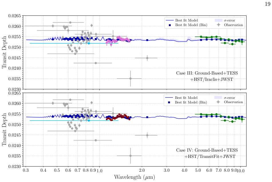
Transit timing variations measured from 188 mid-transit times spanning a decade exhibit no significant evidence of orbital decay. Atmospheric retrievals applied to HST/WFC3 G141 transmission spectra indicate that solutions with higher temperatures are associated with higher water abundances, but combining these spectra with ground-based, TESS, and JWST observations across a wide wavelength range introduces substantial modeling challenges that limit atmospheric characterization.
What carries the argument
Collection and joint analysis of 188 mid-transit times from multi-band observations, together with atmospheric retrieval modeling performed on HST spectra and then extended to broader wavelength datasets.
If this is right
- The orbit of WASP-43 b remains stable with no detectable decay over the ten-year baseline.
- Higher-temperature atmospheric models for this planet correspond to higher water abundances when using HST data alone.
- Broad-wavelength datasets increase the number of free parameters and degeneracies in atmospheric retrievals.
- High-precision, multi-instrument observations will be needed to break current degeneracies in the atmosphere of this target.
Where Pith is reading between the lines
- Similar timing analyses on other short-period hot Jupiters could test whether the lack of decay seen here is typical or exceptional.
- Unquantified instrument-to-instrument differences may affect retrieval results for many exoplanets observed with mixed ground and space facilities.
- Future work could test whether restricting retrievals to narrow, well-calibrated wavelength windows yields more stable abundance estimates before attempting full-spectrum fits.
- Repeated observations with a single stable instrument over time could isolate whether the temperature-water correlation persists independently of dataset combination.
Load-bearing premise
Standard transit-fitting software and atmospheric retrieval models can be applied to observations from different instruments without introducing large unaccounted systematics that alter the combined results.
What would settle it
A new set of transit times collected over the next several years that either shows a clear, steady decrease in orbital period or yields consistent water abundance and temperature values when retrievals are run on uniformly calibrated spectra from all instruments.
Figures


read the original abstract
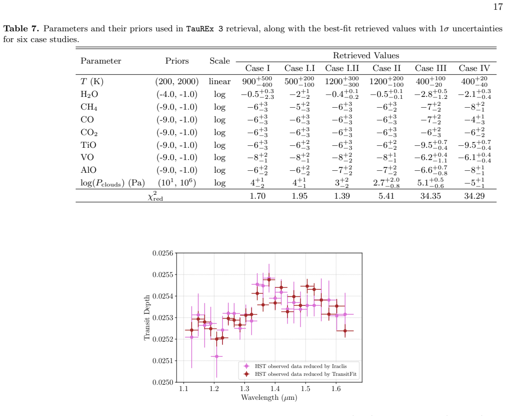
We present a new set of 35 transit light curves of the hot Jupiter WASP-43~b, obtained through the SPEARNET network. These datasets were analyzed together with previously published ground-based observations, as well as space-based data from \emph{TESS}, \emph{HST}, and \emph{JWST}, to refine the planetary parameters of WASP-43~b. A total of 188 mid-transit times, measured with \texttt{TransitFit}, were analyzed for potential timing variations. The transit timing variations do not show any significant evidence of orbital decay. Atmospheric retrievals using \emph{HST}/WFC3 G141 transmission spectra suggest that higher-temperature solutions are associated with higher water abundances. However, when these data are combined with observations from ground-based telescopes, \emph{TESS}, and \emph{JWST}, the increased modeling complexity across the broad wavelength baseline presents significant challenges for atmospheric characterization. These results highlight that high-precision, multi-instrument datasets will be necessary to break existing degeneracies in the atmospheric modeling of this target in the future.
Editorial analysis
A structured set of objections, weighed in public.
Referee Report
Summary. This paper reports 35 new multi-band transit light curves of hot Jupiter WASP-43 b from the SPEARNET network, combined with archival ground-based, TESS, HST, and JWST observations. A total of 188 mid-transit times measured with TransitFit are analyzed for timing variations, yielding no significant evidence of orbital decay. Atmospheric retrievals on HST/WFC3 G141 transmission spectra indicate that higher-temperature solutions correlate with higher water abundances, while noting that combining data across instruments introduces substantial modeling challenges and degeneracies.
Significance. If the results hold, the decade-long timing baseline supplies a clear null detection on orbital decay for this well-studied hot Jupiter, adding to constraints on tidal evolution. The atmospheric section usefully illustrates degeneracies in retrievals and the limits of current multi-instrument datasets. Credit is due for the large homogeneous timing sample, use of standard software (TransitFit) for reproducibility, and the appropriately cautious framing of the HST-only retrieval result rather than overclaiming a multi-instrument solution.
minor comments (3)
- [Abstract] Abstract: the statement that 'higher-temperature solutions are associated with higher water abundances' would be strengthened by a brief parenthetical note on the retrieval code or free parameters used (e.g., whether clouds or metallicity were fixed).
- [TTV analysis] TTV analysis section: while the null result on decay is stated, the manuscript should report the quantitative upper limit on any period derivative (e.g., dP/dt < X s/yr at 3σ) or the likelihood ratio between constant-period and decaying-orbit models to make the 'no significant evidence' claim more precise.
- [Atmospheric retrieval] Atmospheric retrieval section: an explicit statement of how the reported temperature-water correlation was quantified (e.g., Spearman coefficient or marginalized posterior) would help readers evaluate its robustness given the acknowledged degeneracies.
Simulated Author's Rebuttal
We thank the referee for their positive assessment of the manuscript, including recognition of the homogeneous timing sample, use of TransitFit for reproducibility, and the appropriately cautious framing of the HST-only retrieval results. We appreciate the recommendation for minor revision.
Circularity Check
No significant circularity in derivation chain
full rationale
The paper reports direct measurements of 188 mid-transit times from multi-instrument data using the standard TransitFit package, yielding a null result on orbital decay with no claimed detection or tight constraint. Atmospheric retrievals on HST/WFC3 G141 spectra are presented as empirical associations (higher T with higher H2O) accompanied by explicit caveats on degeneracies when combining with ground-based/TESS/JWST data. No steps reduce by construction to fitted inputs, no uniqueness theorems or ansatzes are imported via self-citation, and no predictions are statistically forced from subsets of the same data. All claims derive from external observations and established analysis methods without internal redefinition or load-bearing self-references.
Axiom & Free-Parameter Ledger
axioms (1)
- domain assumption Standard assumptions in transit photometry and atmospheric retrieval hold across instruments
Lean theorems connected to this paper
-
IndisputableMonolith/Foundation/RealityFromDistinction.leanreality_from_one_distinction unclear?
unclearRelation between the paper passage and the cited Recognition theorem.
A total of 188 mid-transit times... analyzed for potential timing variations. The transit timing variations do not show any significant evidence of orbital decay.
-
IndisputableMonolith/Cost/FunctionalEquation.leanwashburn_uniqueness_aczel unclear?
unclearRelation between the paper passage and the cited Recognition theorem.
Atmospheric retrievals using HST/WFC3 G141 transmission spectra suggest that higher-temperature solutions are associated with higher water abundances.
What do these tags mean?
- matches
- The paper's claim is directly supported by a theorem in the formal canon.
- supports
- The theorem supports part of the paper's argument, but the paper may add assumptions or extra steps.
- extends
- The paper goes beyond the formal theorem; the theorem is a base layer rather than the whole result.
- uses
- The paper appears to rely on the theorem as machinery.
- contradicts
- The paper's claim conflicts with a theorem or certificate in the canon.
- unclear
- Pith found a possible connection, but the passage is too broad, indirect, or ambiguous to say the theorem truly supports the claim.
Reference graph
Works this paper leans on
-
[1]
2022, AJ, 163, 77, doi: 10.3847/1538-3881/ac416d
A-thano, N., Jiang, I.-G., Awiphan, S., et al. 2022, AJ, 163, 77, doi: 10.3847/1538-3881/ac416d
-
[2]
Abel, M., Frommhold, L., Li, X., & Hunt, K. L. C. 2011, Journal of Physical Chemistry A, 115, 6805, doi: 10.1021/jp109441f —. 2012, JChPh, 136, 044319, doi: 10.1063/1.3676405
-
[3]
Al-Refaie, A. F., Changeat, Q., Waldmann, I. P., & Tinetti, G. 2021, ApJ, 917, 37, doi: 10.3847/1538-4357/ac0252
-
[4]
2016, MNRAS, 463, 2574, doi: 10.1093/mnras/stw2148
Awiphan, S., Kerins, E., Pichadee, S., et al. 2016, MNRAS, 463, 2574, doi: 10.1093/mnras/stw2148
-
[5]
Bartelt, D., Mansfield, M. W., Line, M. R., et al. 2025, AJ, 169, 101, doi: 10.3847/1538-3881/ad9b95
-
[6]
2022, The Journal of Open Source Software, 7, 4503, doi: 10.21105/joss.04503
Bell, T., Ahrer, E.-M., Brande, J., et al. 2022, The Journal of Open Source Software, 7, 4503, doi: 10.21105/joss.04503
-
[7]
Bell, T. J., Kreidberg, L., Kendrew, S., et al. 2023, arXiv e-prints, arXiv:2301.06350, doi: 10.48550/arXiv.2301.06350
-
[8]
Bell, T. J., Crouzet, N., Cubillos, P. E., et al. 2024, Nature Astronomy, doi: 10.1038/s41550-024-02230-x
-
[9]
Bertin, E., & Arnouts, S. 1996, A&AS, 117, 393, doi: 10.1051/aas:1996164
-
[10]
Blecic, J., Harrington, J., Madhusudhan, N., et al. 2014, ApJ, 781, 116, doi: 10.1088/0004-637X/781/2/116 21 −0.10 −0.05 0.00 0.05 0.10 Phase 0.5 0.6 0.7 0.8 0.9 1.0 Normalized Flux 20190209:0.7-TRT-SBO - I 20190213:0.7-TRT-SBO - I 20190307:0.7-TRT-SBO - I 20190416:0.7-TRT-SBO - I 20200211:0.7-TRT-SBO - R 20210119:0.7-TRT-SBO - R 20210210:0.7-TRT-SBO - R ...
-
[11]
S., Desidera, S., Benatti, S., et al
Bonomo, A. S., Desidera, S., Benatti, S., et al. 2017, A&A, 602, A107, doi: 10.1051/0004-6361/201629882
-
[12]
2021, The Exoplanet Characterization Toolkit (ExoCTK), Zenodo, doi:10.5281/zenodo.4556063
Bourque, M., Espinoza, N., Filippazzo, J., et al. 2021, The Exoplanet Characterization Toolkit (ExoCTK), 1.0.0, Zenodo, doi: 10.5281/zenodo.4556063
-
[13]
2014, A&A, 563, A40, doi: 10.1051/0004-6361/201322740
Chen, G., van Boekel, R., Wang, H., et al. 2014, A&A, 563, A40, doi: 10.1051/0004-6361/201322740
-
[14]
2020, A&A, 639, A3, doi: 10.1051/0004-6361/201937267
Waldmann, I. 2020, A&A, 639, A3, doi: 10.1051/0004-6361/201937267
-
[15]
and Rocchetto, Marco and Yurchenko, Sergei N
Chubb, K. L., Rocchetto, M., Yurchenko, S. N., et al. 2021, A&A, 646, A21, doi: 10.1051/0004-6361/202038350
-
[16]
2000, A&A, 363, 1081
Claret, A. 2000, A&A, 363, 1081
2000
-
[17]
P., et al
Czesla, S., Schr¨ oter, S., Schneider, C. P., et al. 2019, PyA: Python astronomy-related packages. http://ascl.net/1906.010
2019
-
[18]
2021, AJ, 162, 210, doi: 10.3847/1538-3881/ac1baf
Safari, H. 2021, AJ, 162, 210, doi: 10.3847/1538-3881/ac1baf
-
[19]
Deck, K. M., & Agol, E. 2016, ApJ, 821, 96, doi: 10.3847/0004-637X/821/2/96
-
[20]
Dhillon, V. S., Marsh, T. R., Atkinson, D. C., et al. 2014, MNRAS, 444, 4009, doi: 10.1093/mnras/stu1660
-
[21]
Edwards, B., Changeat, Q., Tsiaras, A., et al. 2023, ApJS, 269, 31, doi: 10.3847/1538-4365/ac9f1a
-
[22]
Esposito, M., Covino, E., Desidera, S., et al. 2017, A&A, 601, A53, doi: 10.1051/0004-6361/201629720 22 −0.1 0.0 0.1 Phase 0.80 0.85 0.90 0.95 1.00 Normalized Flux 2013110420131104201311042013110420131104201311042013110420131104201311042013110420131104201311042013110420131104201311042013110420131104201311042013110420131104201311042013110420131104201311042...
-
[23]
Fabrycky, D. C., Ford, E. B., Steffen, J. H., et al. 2012, ApJ, 750, 114, doi: 10.1088/0004-637X/750/2/114
-
[24]
doi:10.1111/j.1365-2966.2009.15598.x , archivePrefix =
Feroz, F., Hobson, M. P., & Bridges, M. 2009, MNRAS, 398, 1601, doi: 10.1111/j.1365-2966.2009.14548.x
-
[25]
N., Gustafsson, M., & Orton, G
Fletcher, L. N., Gustafsson, M., & Orton, G. S. 2018, ApJS, 235, 24, doi: 10.3847/1538-4365/aaa07a
-
[26]
and Lang, Dustin and Goodman, Jonathan , title =
Foreman-Mackey, D., Hogg, D. W., Lang, D., & Goodman, J. 2013, PASP, 125, 306, doi: 10.1086/670067
-
[27]
Fulton, B. J., Shporer, A., Winn, J. N., et al. 2011, The Astronomical Journal, 142, 84, doi: 10.1088/0004-6256/142/3/84
-
[28]
2021, MNRAS, 508, 5514, doi: 10.1093/mnras/stab2929
Garai, Z., Pribulla, T., Parviainen, H., et al. 2021, MNRAS, 508, 5514, doi: 10.1093/mnras/stab2929
-
[29]
Gillon, M., Triaud, A. H. M. J., Fortney, J. J., et al. 2012, A&A, 542, A4, doi: 10.1051/0004-6361/201218817
-
[30]
S., Wilzewski, J
Gordon, I., Rothman, L. S., Wilzewski, J. S., et al. 2016, in AAS/Division for Planetary Sciences Meeting Abstracts, Vol. 48, AAS/Division for Planetary Sciences Meeting Abstracts #48, 421.13
2016
-
[31]
Grant, D., Lewis, N. K., Wakeford, H. R., et al. 2023, ApJL, 956, L32, doi: 10.3847/2041-8213/acfc3b10.3847/2041-8213/acfdab
work page doi:10.3847/2041-8213/acfc3b10.3847/2041-8213/acfdab 2023
-
[32]
Hayes, J. J. C., Priyadarshi, A., Kerins, E., et al. 2024, MNRAS, 527, 4936, doi: 10.1093/mnras/stad3353
-
[33]
R., Collier Cameron, A., et al
Hellier, C., Anderson, D. R., Collier Cameron, A., et al. 2011, A&A, 535, L7, doi: 10.1051/0004-6361/201117081
-
[34]
2016, AJ, 151, 137, doi: 10.3847/0004-6256/151/6/137
Hoyer, S., Pall´ e, E., Dragomir, D., & Murgas, F. 2016, AJ, 151, 137, doi: 10.3847/0004-6256/151/6/137
-
[35]
2013, A&A, 553, A6, doi: 10.1051/0004-6361/201219058
Husser, T. O., Wende-von Berg, S., Dreizler, S., et al. 2013, A&A, 553, A6, doi: 10.1051/0004-6361/201219058
-
[36]
Ivshina, E. S., & Winn, J. N. 2022, ApJS, 259, 62, doi: 10.3847/1538-4365/ac545b
-
[37]
M., et al., 2016, in Chiozzi G., Guzman J
Jenkins, J. M., Twicken, J. D., McCauliff, S., et al. 2016, in Society of Photo-Optical Instrumentation Engineers (SPIE) Conference Series, Vol. 9913, Software and Cyberinfrastructure for Astronomy IV, ed. G. Chiozzi & J. C. Guzman, 99133E, doi: 10.1117/12.2233418
-
[38]
2016, AJ, 151, 17, doi: 10.3847/0004-6256/151/1/17
Jiang, I.-G., Lai, C.-Y., Savushkin, A., et al. 2016, AJ, 151, 17, doi: 10.3847/0004-6256/151/1/17
-
[39]
2018, Research Notes of the AAS, 2, 4, doi: 10.3847/2515-5172/aaa4b7
Kanodia, S., & Wright, J. 2018, Research Notes of the AAS, 2, 4, doi: 10.3847/2515-5172/aaa4b7
-
[40]
2023, ApJS, 265, 4, doi: 10.3847/1538-4365/ac9da4
Kokori, A., Tsiaras, A., Edwards, B., et al. 2023, ApJS, 265, 4, doi: 10.3847/1538-4365/ac9da4
-
[41]
2015, Publications of the Astronomical Society of the Pacific, 127, 1161, doi: 10.1086/683602
Kreidberg, L. 2015, PASP, 127, 1161, doi: 10.1086/683602
-
[42]
Kreidberg, L., Line, M. R., Thorngren, D., Morley, C. V., & Stevenson, K. B. 2018, ApJL, 858, L6, doi: 10.3847/2041-8213/aabfce
-
[43]
Kreidberg, L., Bean, J. L., D´ esert, J.-M., et al. 2014, ApJL, 793, L27, doi: 10.1088/2041-8205/793/2/L27
-
[44]
W., Mierle, K., Blanton, M., & Roweis, S
Lang, D., Hogg, D. W., Mierle, K., Blanton, M., & Roweis, S. 2010, AJ, 139, 1782, doi: 10.1088/0004-6256/139/5/1782
-
[45]
2023, A&A, 678, A23, doi: 10.1051/0004-6361/202347151
Lesjak, F., Nortmann, L., Yan, F., et al. 2023, A&A, 678, A23, doi: 10.1051/0004-6361/202347151
-
[46]
2013, Information Bulletin on Variable Stars, 6082, 1
Maciejewski, G., Puchalski, D., Saral, G., et al. 2013, Information Bulletin on Variable Stars, 6082, 1
2013
-
[47]
McDonald, I., van Loon, J. T., Decin, L., et al. 2009, MNRAS, 394, 831, doi: 10.1111/j.1365-2966.2008.14370.x
-
[48]
McDonald, I., Zijlstra, A. A., & Boyer, M. L. 2012, MNRAS, 427, 343, doi: 10.1111/j.1365-2966.2012.21873.x
-
[49]
McDonald, I., Zijlstra, A. A., & Watson, R. A. 2017, MNRAS, 471, 770, doi: 10.1093/mnras/stx1433
-
[50]
K., Masseron, T., Hoeijmakers, H
McKemmish, L. K., Masseron, T., Hoeijmakers, H. J., et al. 2019, MNRAS, 488, 2836, doi: 10.1093/mnras/stz1818
-
[51]
McKemmish, L. K., Yurchenko, S. N., & Tennyson, J. 2016, MNRAS, 463, 771, doi: 10.1093/mnras/stw1969
-
[52]
Murgas, F., Pall´ e, E., Zapatero Osorio, M. R., et al. 2014, A&A, 563, A41, doi: 10.1051/0004-6361/201322374
-
[53]
Parviainen, H., Tingley, B., Deeg, H. J., et al. 2019, A&A, 630, A89, doi: 10.1051/0004-6361/201935709
-
[54]
Patra, K. C., Winn, J. N., Holman, M. J., et al. 2020, AJ, 159, 150, doi: 10.3847/1538-3881/ab7374
-
[55]
T., Hill, C., Tennyson, J., & Yurchenko, S
Patrascu, A. T., Hill, C., Tennyson, J., & Yurchenko, S. N. 2014, The Journal of Chemical Physics, 141, 144312, doi: 10.1063/1.4897484
-
[56]
Polyansky, O. L., Kyuberis, A. A., Zobov, N. F., et al. 2018, MNRAS, 480, 2597, doi: 10.1093/mnras/sty1877
-
[57]
Ricci, D., Ram´ on-Fox, F. G., Ayala-Loera, C., et al. 2015, PASP, 127, 143, doi: 10.1086/680233
-
[58]
Rothman, L. S., & Gordon, I. E. 2014, in 13th International HITRAN Conference, 49, doi: 10.5281/zenodo.11207
-
[59]
Speagle, J. S. 2020, MNRAS, 493, 3132, doi: 10.1093/mnras/staa278
-
[60]
Stevenson, K. B., Line, M. R., Bean, J. L., et al. 2017, AJ, 153, 68, doi: 10.3847/1538-3881/153/2/68
-
[61]
Tennyson, J., Yurchenko, S. N., Al-Refaie, A. F., et al. 2016, Journal of Molecular Spectroscopy, 327, 73, doi: 10.1016/j.jms.2016.05.002
-
[62]
Instrumentation in astronomy VI , year = 1986, editor =
Tody, D. 1986, in Society of Photo-Optical Instrumentation Engineers (SPIE) Conference Series, Vol. 627, Instrumentation in astronomy VI, ed. D. L. Crawford, 733, doi: 10.1117/12.968154
-
[63]
1993, in Astronomical Society of the Pacific Conference Series, Vol
Tody, D. 1993, in Astronomical Society of the Pacific Conference Series, Vol. 52, Astronomical Data Analysis Software and Systems II, ed. R. J. Hanisch, R. J. V. Brissenden, & J. Barnes, 173
1993
-
[64]
Tsiaras, A., Waldmann, I. P., Rocchetto, M., et al. 2016a, ApJ, 832, 202, doi: 10.3847/0004-637X/832/2/202 24 −0.05 0.00 0.05 Phase −0.2 0.0 0.2 0.4 0.6 0.8 1.0 Normalized Flux TESS Sector 35 TESS Sector 35 TESS Sector 35 TESS Sector 35 TESS Sector 35 TESS Sector 35 TESS Sector 35 TESS Sector 35 TESS Sector 35 TESS Sector 35 TESS Sector 35 TESS Sector 35 ...
-
[65]
Tsiaras, A., Rocchetto, M., Waldmann, I. P., et al. 2016c, ApJ, 820, 99, doi: 10.3847/0004-637X/820/2/99
-
[66]
Tsiaras, A., Waldmann, I. P., Zingales, T., et al. 2018, AJ, 155, 156, doi: 10.3847/1538-3881/aaaf75
-
[67]
C., L´ opez-Morales, M., Espinoza, N., et al
Weaver, I. C., L´ opez-Morales, M., Espinoza, N., et al. 2020, AJ, 159, 13, doi: 10.3847/1538-3881/ab55da
-
[68]
2020, AJ, 160, 155, doi: 10.3847/1538-3881/ababad
Wong, I., Shporer, A., Daylan, T., et al. 2020, AJ, 160, 155, doi: 10.3847/1538-3881/ababad
-
[69]
Tennyson, J. 2020, MNRAS, 496, 5282, doi: 10.1093/mnras/staa1874
-
[70]
N., Owens, A., Kefala, K., & Tennyson, J
Yurchenko, S. N., Owens, A., Kefala, K., & Tennyson, J. 2024, MNRAS, 528, 3719, doi: 10.1093/mnras/stae148
-
[71]
Zechmeister, M., & K¨ urster, M. 2009, A&A, 496, 577, doi: 10.1051/0004-6361:200811296 26 −4.5 −3.0 −1.5 log10(H2O) −8 −6 −4 −2 log10(CH4) −8 −6 −4 −2 log10(CO) −8 −6 −4 −2 log10(CO2) −8 −6 −4 −2 log10(TiO) −8 −6 −4 −2 log10(VO) −8 −6 −4 −2 log10(AlO) 400 800120016002000 Tp 2 3 4 5 6 log10(P c) −4.5 −3.0 −1.5 log10(H2O) −8 −6 −4 −2 log10(CH4) −8 −6 −4 −2 ...
discussion (0)
Sign in with ORCID, Apple, or X to comment. Anyone can read and Pith papers without signing in.