Recognition: 3 theorem links
· Lean TheoremHidden in Plain Sight: Visual-to-Symbolic Analytical Solution Inference from Field Visualizations
Pith reviewed 2026-05-10 18:18 UTC · model grok-4.3
The pith
A vision-language model recovers exact symbolic equations from images of physical fields.
A machine-rendered reading of the paper's core claim, the machinery that carries it, and where it could break.
Core claim
ViSA-R2 demonstrates that aligning a vision-language model with a structured, solution-centric chain-of-thought pipeline enables accurate recovery of executable symbolic analytical solutions from visualizations of linear steady-state fields, outperforming other models under a standardized evaluation protocol on the released ViSA-Bench.
What carries the argument
The self-verifying, solution-centric chain-of-thought pipeline that proceeds through structural pattern recognition, solution-family hypothesis, parameter derivation, and consistency verification.
Load-bearing premise
That the 30 synthetic linear steady-state scenarios with perfect annotations sufficiently represent the noise, complexity, and ambiguity present in real-world visual observations of physical fields.
What would settle it
Run the model on real experimental images of physical fields that contain sensor noise, incomplete views, or non-ideal boundary conditions and measure whether the output SymPy expressions still match ground-truth solutions within numerical tolerance.
Figures


read the original abstract
Recovering analytical solutions of physical fields from visual observations is a fundamental yet underexplored capability for AI-assisted scientific reasoning. We study visual-to-symbolic analytical solution inference (ViSA) for two-dimensional linear steady-state fields: given field visualizations (and first-order derivatives) plus minimal auxiliary metadata, the model must output a single executable SymPy expression with fully instantiated numeric constants. We introduce ViSA-R2 and align it with a self-verifying, solution-centric chain-of-thought pipeline that follows a physicist-like pathway: structural pattern recognition solution-family (ansatz) hypothesis parameter derivation consistency verification. We also release ViSA-Bench, a VLM-ready synthetic benchmark covering 30 linear steady-state scenarios with verifiable analytical/symbolic annotations, and evaluate predictions by numerical accuracy, expression-structure similarity, and character-level accuracy. Using an 8B open-weight Qwen3-VL backbone, ViSA-R2 outperforms strong open-source baselines and the evaluated closed-source frontier VLMs under a standardized protocol.
Editorial analysis
A structured set of objections, weighed in public.
Referee Report
Summary. The paper introduces ViSA-R2, an 8B Qwen3-VL-based model using a self-verifying, physicist-inspired chain-of-thought pipeline (structural pattern recognition, ansatz hypothesis, parameter derivation, consistency verification) to infer executable SymPy analytical expressions from visualizations of 2D linear steady-state fields plus derivatives and metadata. It releases ViSA-Bench, a synthetic VLM-ready benchmark of 30 scenarios with verifiable symbolic annotations, and reports that ViSA-R2 outperforms open-source baselines and evaluated closed-source VLMs on numerical accuracy, expression-structure similarity, and character-level accuracy under a standardized protocol.
Significance. If the outperformance holds under a fully specified protocol, the work would advance AI-assisted scientific reasoning by showing how VLMs can recover fully instantiated symbolic solutions from visual field data in a structured manner. The release of ViSA-Bench and reliance on an open-weight backbone are strengths for reproducibility and follow-up work. The contribution is scoped to synthetic linear steady-state cases, so its significance for broader physical-field inference depends on demonstrated generalization beyond the current benchmark.
major comments (2)
- [Abstract and Experiments section] Abstract and evaluation protocol: The central claim of outperformance on numerical accuracy, expression-structure similarity, and character-level accuracy is asserted without any quantitative results, error bars, ablation on post-hoc filtering, or explicit definition of how the three metrics are computed and aggregated. This omission is load-bearing because it prevents verification of the magnitude and robustness of the reported gains over baselines.
- [Benchmark section] ViSA-Bench construction (§ on benchmark): The evaluation rests on 30 synthetic linear steady-state scenarios with perfect annotations. While this enables verifiable ground truth, the paper does not demonstrate that this scale and idealized construction (no sensor noise, ambiguity, or higher-order nonlinearities) is independent of the method's assumptions or sufficient to support claims about real-world visual observations of physical fields.
Simulated Author's Rebuttal
We thank the referee for the detailed and constructive report. We address each major comment below, indicating where we will revise the manuscript to improve clarity and completeness while preserving the stated scope of the work.
read point-by-point responses
-
Referee: [Abstract and Experiments section] Abstract and evaluation protocol: The central claim of outperformance on numerical accuracy, expression-structure similarity, and character-level accuracy is asserted without any quantitative results, error bars, ablation on post-hoc filtering, or explicit definition of how the three metrics are computed and aggregated. This omission is load-bearing because it prevents verification of the magnitude and robustness of the reported gains over baselines.
Authors: We agree that the abstract currently states outperformance without numerical values and that the main text would benefit from more explicit metric definitions and protocol details. In the revised manuscript we will (1) insert the primary quantitative results (mean numerical accuracy, expression-structure similarity, and character-level accuracy with standard deviations across runs) into the abstract, (2) add a dedicated subsection in Experiments that formally defines each metric (numerical accuracy as mean relative L2 error on a 100×100 evaluation grid, expression-structure similarity via normalized tree-edit distance on SymPy ASTs, character-level accuracy via normalized Levenshtein distance), (3) report an ablation isolating the contribution of the post-hoc consistency filter, and (4) expand the evaluation protocol description to include exact prompting templates, sampling parameters, and aggregation rules used for all models. These additions will make the magnitude and robustness of the gains directly verifiable. revision: yes
-
Referee: [Benchmark section] ViSA-Bench construction (§ on benchmark): The evaluation rests on 30 synthetic linear steady-state scenarios with perfect annotations. While this enables verifiable ground truth, the paper does not demonstrate that this scale and idealized construction (no sensor noise, ambiguity, or higher-order nonlinearities) is independent of the method's assumptions or sufficient to support claims about real-world visual observations of physical fields.
Authors: The manuscript explicitly limits its claims to synthetic 2D linear steady-state fields and presents ViSA-Bench as a controlled, verifiable testbed rather than a proxy for real-world data. The 30 scenarios were deliberately constructed to cover a representative range of common linear operators and boundary conditions while guaranteeing perfect symbolic ground truth. We acknowledge that this idealized setting does not yet address sensor noise or nonlinearities. In revision we will expand the Limitations and Future Work section to (a) articulate why the current scale and construction are sufficient to validate the core self-verifying pipeline, (b) discuss the independence of the benchmark from the method’s assumptions, and (c) outline concrete next steps for introducing controlled noise and nonlinear PDE cases. No claim of immediate real-world sufficiency is made in the present work. revision: partial
Circularity Check
No significant circularity in derivation chain
full rationale
The paper's central contribution is an empirical VLM-based pipeline (ViSA-R2) evaluated for outperformance on a released synthetic benchmark (ViSA-Bench) of 30 linear steady-state field scenarios with independent verifiable analytical annotations. No load-bearing mathematical derivation, parameter fitting, or uniqueness theorem is present that reduces outputs to inputs by construction. The described self-verifying CoT pathway follows an explicit physicist-like sequence (pattern recognition → ansatz hypothesis → parameter derivation → consistency check) without self-definitional loops or renaming of known results. Self-citations, if any, are not invoked to justify uniqueness or forbid alternatives. The benchmark supplies external ground truth independent of the model's predictions, satisfying the criteria for a non-circular empirical claim.
Axiom & Free-Parameter Ledger
axioms (2)
- domain assumption The target fields are two-dimensional linear steady-state phenomena whose solutions belong to recognizable analytical families.
- domain assumption First-order derivatives plus minimal auxiliary metadata are sufficient to disambiguate solution parameters.
invented entities (2)
-
ViSA-R2
no independent evidence
-
ViSA-Bench
no independent evidence
Lean theorems connected to this paper
-
IndisputableMonolith/Cost/FunctionalEquation.leanwashburn_uniqueness_aczel unclear?
unclearRelation between the paper passage and the cited Recognition theorem.
structural pattern recognition → solution-family (ansatz) hypothesis → parameter derivation → consistency verification
-
IndisputableMonolith/Foundation/RealityFromDistinction.leanreality_from_one_distinction unclear?
unclearRelation between the paper passage and the cited Recognition theorem.
30 linear steady-state scenarios with verifiable analytical/symbolic annotations
-
IndisputableMonolith/Foundation/AlexanderDuality.leanalexander_duality_circle_linking unclear?
unclearRelation between the paper passage and the cited Recognition theorem.
ViSA-R2 outperforms ... under a standardized protocol on ViSA-Bench
What do these tags mean?
- matches
- The paper's claim is directly supported by a theorem in the formal canon.
- supports
- The theorem supports part of the paper's argument, but the paper may add assumptions or extra steps.
- extends
- The paper goes beyond the formal theorem; the theorem is a base layer rather than the whole result.
- uses
- The paper appears to rely on the theorem as machinery.
- contradicts
- The paper's claim conflicts with a theorem or certificate in the canon.
- unclear
- Pith found a possible connection, but the passage is too broad, indirect, or ambiguous to say the theorem truly supports the claim.
Reference graph
Works this paper leans on
-
[1]
MME: A Comprehensive Evaluation Benchmark for Multimodal Large Language Models
URL https://openreview.net/forum? id=DgH9YCsqWm. Spotlight. arXiv:2306.13394. Gao, L., Madaan, A., Zhou, S., Alon, U., Liu, P., Yang, Y ., Callan, J., and Neubig, G. PAL: Program-aided language models. InProceedings of the 40th International Confer- ence on Machine Learning, volume 202 ofProceedings of Machine Learning Research, pp. 10764–10799. PMLR,
work page internal anchor Pith review arXiv
-
[2]
XNOR-Net: ImageNet Classification Using Binary Convolutional Neural Networks , booktitle =
URL https://proceedings.mlr.press/ v202/gao23f.html. Google DeepMind. Gemini 3 pro. Model re- lease, 2025. URL https://deepmind.google/ models/gemini/pro/. Large language model. Ac- cessed 2026-01-29. Kafle, K., Price, B., Cohen, S., and Kanan, C. DVQA: Understanding data visualizations via question answering. InProceedings of the IEEE Confer- ence on Com...
-
[3]
Li, D., Yin, J., Xu, J., Li, X., and Zhang, J
Curran Associates, Inc., 2022. Li, D., Yin, J., Xu, J., Li, X., and Zhang, J. Visymre: Vision-guided multimodal symbolic regression.arXiv preprint arXiv:2412.11139, 2024. URL https:// arxiv.org/abs/2412.11139. Li, J., Li, D., Savarese, S., and Hoi, S. BLIP-2: Bootstrap- ping language-image pre-training with frozen image en- coders and large language model...
-
[4]
doi: 10.1007/ 978-3-031-72658-3 13
Springer Nature Switzerland, 2024. doi: 10.1007/ 978-3-031-72658-3 13. URL https://doi.org/ 10.1007/978-3-031-72658-3_13. Lu, P., Mishra, S., Xia, T., Qiu, L., Chang, K.-W., Zhu, S.-C., Tafjord, O., Clark, P., and Kalyan, A. Learn to explain: Multimodal reasoning via thought chains for science question answering. InAdvances in Neural Infor- mation Process...
-
[5]
URL https://openaccess.thecvf. com/content_WACV_2020/html/Methani_ PlotQA_Reasoning_over_Scientific_ Plots_WACV_2020_paper.html. OpenAI. Gpt-5.2. Model release, 2025. URL https:// openai.com/index/introducing-gpt-5-2/ . Large language model. Accessed 2026-01-29. Schick, T., Dwivedi-Yu, J., Dessi, R., Raileanu, R., Lomeli, M., Hambro, E., Zettlemoyer, L., ...
-
[6]
URL https://proceedings.mlr.press/ v235/wang24z.html. xAI. Grok 4.1. Model release, 2025a. URL https: //x.ai/news/grok-4-1. Large language model. Accessed 2026-01-29. xAI. Grok 4. Model release, 2025b. URL https://x. ai/news/grok-4. Large language model. Accessed 2026-01-29. Xu, X., Xu, Q., Xiao, T., Chen, T., Yan, Y ., Zhang, J., Diao, S., Yang, C., and ...
-
[7]
PhysReason: A comprehensive benchmark towards physics-based reasoning
URL https://openaccess.thecvf. com/content/CVPR2024/html/Yue_MMMU_A_ Massive_Multi-discipline_Multimodal_ Understanding_and_Reasoning_ Benchmark_for_CVPR_2024_paper.html. Zhang, H., Chen, Q., Xue, B., Banzhaf, W., and Zhang, M. RAG-SR: Retrieval-augmented generation for neural symbolic regression. InInternational Conference on Learning Representations (IC...
-
[8]
Describe the overall pattern/shape of the scalar field
-
[9]
Identify any special features: symmetries, extrema, zeros, singularities, boundaries
-
[10]
Read values from the colorbars to estimate: • Maximum and minimum values ofu(x, y) • Approximate values of∂u/∂xand∂u/∂y
-
[11]
Prompt: You are analyzing numerical data for a scalar fieldu(x, y)over domain[x min,x max,y min,y max]
Note any special behaviors: radial patterns, linear gradients, oscillations, decay patterns Output format: SUMMARY: - Pattern: [concise description] - Symmetry: [none/radial/translational/rotational/other] - Max value: [estimate from colorbar] - Min value: [estimate from colorbar] - Gradient type: [uniform/varying/radial/other] - Special features: [list k...
-
[12]
Verify the image observations with numerical data
-
[13]
Calculate key numerical metrics (range, gradients, extrema locations)
-
[14]
Identify numerical patterns (decay rates, oscillation frequencies, radial profiles)
-
[15]
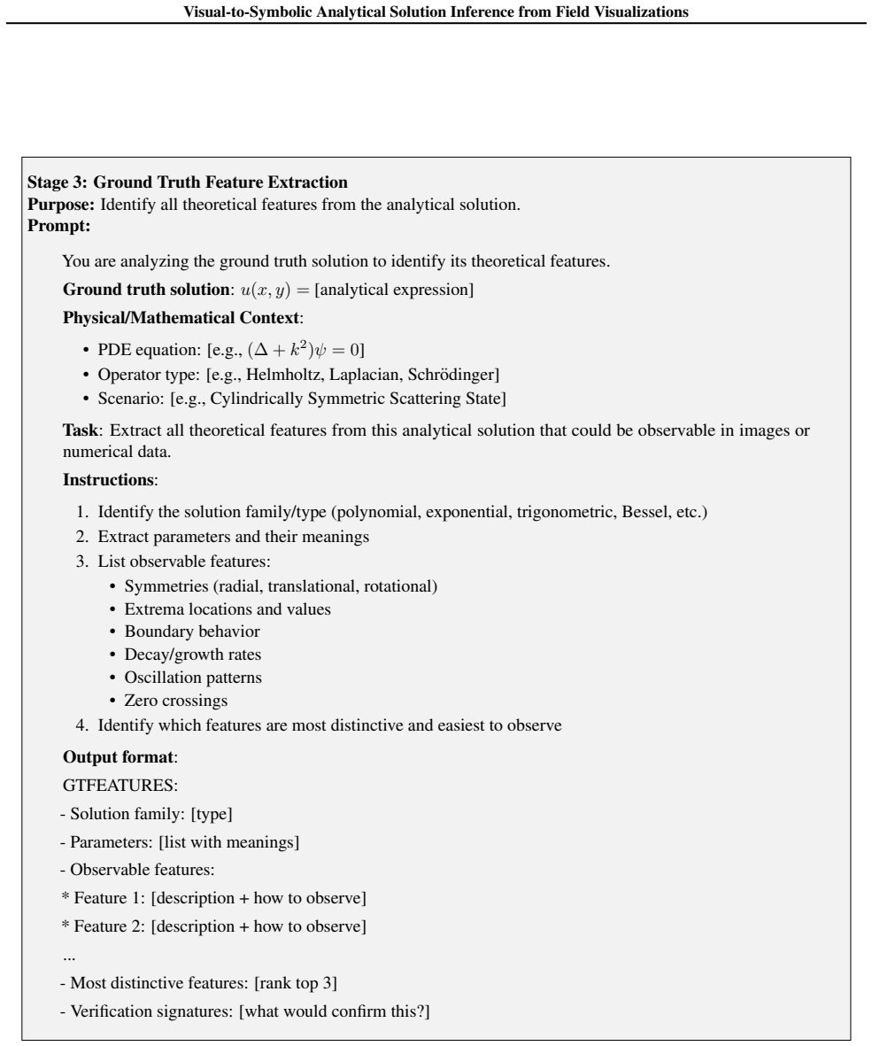
Prompt: You are analyzing the ground truth solution to identify its theoretical features
Look for quantitative clues about the solution form Output format: NUMERICAL EVIDENCE: • Max: [value] at approximately [location] • Min: [value] at approximately [location] • Gradient magnitude: [range] • Decay/growth rate: [estimate if applicable] • Oscillation frequency: [estimate if applicable] • Key ratios: [any useful ratios between quantities] Figur...
-
[16]
Identify the solution family/type (polynomial, exponential, trigonometric, Bessel, etc.)
-
[17]
Extract parameters and their meanings
-
[18]
List observable features: • Symmetries (radial, translational, rotational) • Extrema locations and values • Boundary behavior • Decay/growth rates • Oscillation patterns • Zero crossings
-
[19]
Identify which features are most distinctive and easiest to observe Output format: GTFEATURES: - Solution family: [type] - Parameters: [list with meanings] - Observable features: * Feature 1: [description + how to observe] * Feature 2: [description + how to observe] ... - Most distinctive features: [rank top 3] - Verification signatures: [what would confi...
-
[20]
Which GT features are clearly present in observations
-
[21]
Which GT features are ambiguous or hard to confirm
-
[22]
Any contradictions that need resolution Instructions:
-
[23]
For each GT feature, check if it appears in Stage 1 or Stage 2 observations
-
[24]
Rate the match quality: STRONG MODERATE WEAK ABSENT CONTRADICTORY
-
[25]
Identify which parameters can be estimated from which observations
-
[26]
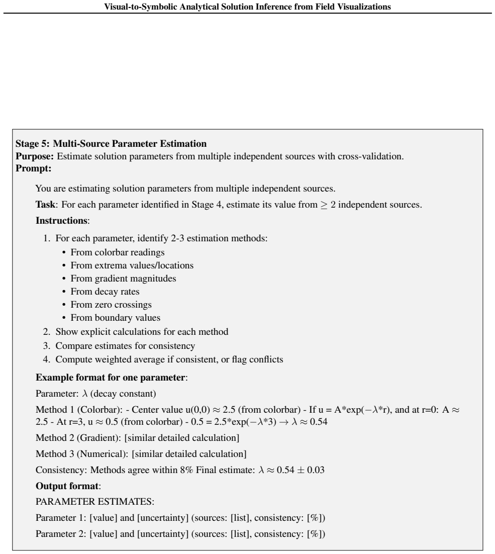
Prompt: You are estimating solution parameters from multiple independent sources
Flag any inconsistencies between images and numerical data Output format: FEATUREMATCHING: Confirmed features (STRONG match): - [Feature]: [evidence from Stage 1 2] Probable features (MODERATE match): - [Feature]: [evidence from Stage 1 2] Unclear features (WEAK/ABSENT): - [Feature]: [why unclear] Contradictions: - [Any contradictions and potential resolu...
-
[27]
For each parameter, identify 2-3 estimation methods: • From colorbar readings • From extrema values/locations • From gradient magnitudes • From decay rates • From zero crossings • From boundary values
-
[28]
Show explicit calculations for each method
-
[29]
Compare estimates for consistency
-
[30]
Prompt: You are generating a Chain-of-Thought (CoT) reasoning process for predicting a PDE solution
Compute weighted average if consistent, or flag conflicts Example format for one parameter: Parameter:λ(decay constant) Method 1 (Colorbar): - Center value u(0,0) ≈ 2.5 (from colorbar) - If u = A*exp(−λ*r), and at r=0: A ≈ 2.5 - At r=3, u≈0.5 (from colorbar) - 0.5 = 2.5*exp(−λ*3)→λ≈0.54 Method 2 (Gradient): [similar detailed calculation] Method 3 (Numeric...
-
[31]
Starts from observations (what you see in images/data)
-
[32]
Identifies patterns and makes hypotheses about solution type
-
[33]
Estimates parameters through explicit calculations
-
[34]
Arrives at the final solution
-
[35]
the ground truth is
Verifies the solution makes sense Critical requirements: • Use natural language (like human reasoning, not JSON) • Show explicit arithmetic calculations • Use multi-source parameter verification • DO NOT say “the ground truth is...” or “comparing with GT...” • Make it seem like independent reasoning from observations • The CoT should lead naturally to the...
-
[36]
From colorbar: center value A≈2.5
-
[37]
From decay: at r≈3, u≈0.5, so 0.5 = 2.5 *exp(-3λ)→λ≈0.536
-
[38]
[continue reasoning with calculations] </thinking> <solution>[final SymPy expression]</solution> The CoT should be 300–800 words, showing detailed step-by-step reasoning
Verification from gradient: ... [continue reasoning with calculations] </thinking> <solution>[final SymPy expression]</solution> The CoT should be 300–800 words, showing detailed step-by-step reasoning. Figure 9.Stage 6: Chain-of-Thought Generation Prompt 18 Visual-to-Symbolic Analytical Solution Inference from Field Visualizations Test Prompt: Direct Sym...
-
[39]
Scalar Field Visualization The first image shows the scalar fieldu(x, y)as a heatmap
-
[40]
Gradient Components Visualization The second image shows the gradient components∂u/∂xand∂u/∂y
-
[41]
Field Data (CSV) Data shape: (400, 3) Columns: x, y, u Value ranges: x: [xmin, xmax] y: [ymin, ymax] u: [umin, umax] First 10 rows: x y u [data rows...]
-
[42]
Required Output Format Your response MUST follow this exact structure: <thinking> Provide your detailed reasoning process here:
Gradient Data (CSV) Data shape: (400, 4) Columns: x, y, du dx, du dy Value ranges: x: [xmin, xmax] y: [ymin, ymax] du dx: [grad x min, grad x max] du dy: [grad y min, grad y max] First 10 rows: x y du dx du dy [data rows...] Task Based on the visualizations and numerical data above, derive the symbolic expression for the scalar field u(x, y). Required Out...
-
[43]
Analyze the patterns, symmetries, and mathematical properties observed
-
[44]
Identify key features (e.g., radial symmetry, polynomial behavior, special functions)
-
[45]
Propose candidate symbolic expressions
-
[46]
Verify hypotheses against the observed data
-
[47]
Examples: - x **2 + y **2 - sin(x) *cos(y) - exp(-x **2 - y **2) - besselj(0, sqrt(x **2 + y **2)) </solution> Figure 10.Test/Inference Prompt for Symbolic Regression Evaluation 19
Refine the solution based on verification results </thinking> <solution> Provide the final symbolic expression in SymPy format. Examples: - x **2 + y **2 - sin(x) *cos(y) - exp(-x **2 - y **2) - besselj(0, sqrt(x **2 + y **2)) </solution> Figure 10.Test/Inference Prompt for Symbolic Regression Evaluation 19
discussion (0)
Sign in with ORCID, Apple, or X to comment. Anyone can read and Pith papers without signing in.