arxiv: 2604.09346 · v1 · submitted 2026-04-10 · ⚛️ physics.ao-ph

Recognition: unknown

OTProf: estimating high-resolution profiles of optical turbulence (C_n²) from reanalysis using deep learning

Maximilian Pierzyna , Sukanta Basu , Rudolf Saathof

Authors on Pith no claims yet

Pith reviewed 2026-05-10 16:04 UTC · model grok-4.3

classification ⚛️ physics.ao-ph

keywords optical turbulenceCn2 profilesdeep learningERA5 reanalysisFried parameterscintillation indexHufnagel-Valley modelatmospheric optics

0 comments

The pith

Deep learning produces better Cn2 profiles than Hufnagel-Valley from reanalysis

A machine-rendered reading of the paper's core claim, the machinery that carries it, and where it could break.

The paper presents OTProf, a deep learning method that turns coarse ERA5 reanalysis data into high-resolution vertical profiles of optical turbulence strength Cn². Accurate profiles matter for ground-based astronomy and free-space optical communication because turbulence affects image quality and signal strength, yet obtaining them through direct measurement or detailed simulations is resource-intensive. OTProf learns the statistical connection between broad meteorological variables and fine-scale turbulence, reproducing vertical structures more accurately than the standard Hufnagel-Valley model and delivering improved values for the integrated Fried parameter r0 and scintillation index σ_I². The outputs remain physically consistent overall, though they smooth some rare strong turbulence peaks, which can make certain performance estimates slightly optimistic. The approach provides an efficient alternative once the model is trained.

Core claim

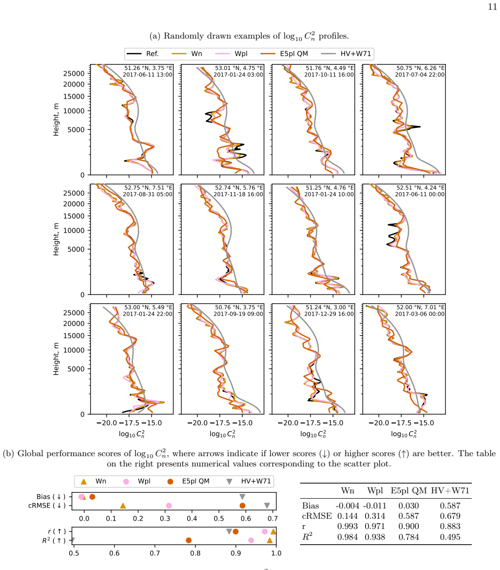
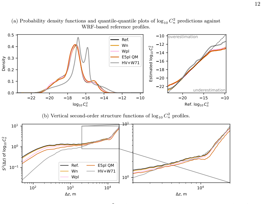
OTProf is a deep-learning method that estimates high-resolution Cn² profiles from coarse-resolution ERA5 reanalysis data. When evaluated in the Netherlands, it reproduces the vertical structure of Cn² more accurately than the Hufnagel-Valley model and yields more accurate estimates of the Fried parameter r0 and the scintillation index σ_I². The Cn² predictions are slightly smoothed compared to reference data, especially in cases of rare strong turbulence. This smoothing affects the integrated parameters, sometimes leading to overly optimistic r0 and σ_I² values. Despite this, OTProf offers a more accurate, efficient, and physically consistent alternative to traditional analytical models and

What carries the argument

OTProf, a neural network trained to map coarse meteorological fields from ERA5 reanalysis to high-resolution Cn² profiles.

If this is right

OTProf supplies location-specific high-resolution turbulence profiles without the computational cost of mesoscale numerical weather models.
It improves accuracy for the Fried parameter r0, a measure of atmospheric coherence length, and the scintillation index σ_I², which quantifies intensity fluctuations.
The method serves as a practical alternative to analytical models for designing optical systems in astronomy and communications.
After training, new reanalysis data can be processed rapidly to support historical or near-real-time turbulence analysis.

Where Pith is reading between the lines

These are editorial extensions of the paper, not claims the author makes directly.

Retraining or adapting OTProf on data from other regions could enable creation of global turbulence profile archives from existing reanalysis records.
The observed smoothing of strong turbulence events suggests that adding uncertainty quantification or ensemble predictions could further improve extreme-value accuracy.
Similar data-driven mappings might be applied to estimate other hard-to-resolve atmospheric optical parameters from standard weather reanalysis.

Load-bearing premise

The statistical relationship learned from training data in the Netherlands is physically consistent and generalizes to other locations and conditions without significant domain shift.

What would settle it

Comparing OTProf Cn² profiles against independent high-resolution measurements collected at a site outside the Netherlands with different topography or climate would show whether the accuracy advantage over Hufnagel-Valley holds.

Figures

Figures reproduced from arXiv: 2604.09346 by Maximilian Pierzyna, Rudolf Saathof, Sukanta Basu.

**Figure 2.** Figure 2: FIG. 2: Overview of training and inference pipeline of OTProf utilizing the Squeezeformer architecture. [PITH_FULL_IMAGE:figures/full_fig_p003_2.png] view at source ↗

**Figure 3.** Figure 3: FIG. 3: Horizontal (a and b) and vertical (c) extent of [PITH_FULL_IMAGE:figures/full_fig_p007_3.png] view at source ↗

**Figure 4.** Figure 4: FIG. 4: Visual and statistical comparison of predicted [PITH_FULL_IMAGE:figures/full_fig_p011_4.png] view at source ↗

**Figure 5.** Figure 5: FIG. 5: Statistical characteristics of predicted [PITH_FULL_IMAGE:figures/full_fig_p012_5.png] view at source ↗

**Figure 6.** Figure 6: FIG. 6: Performance scores, histograms, and quantile-quantile plots for the integrated OT parameters [PITH_FULL_IMAGE:figures/full_fig_p013_6.png] view at source ↗

**Figure 7.** Figure 7: FIG. 7: Performance scores and statistical characteristics of predicted [PITH_FULL_IMAGE:figures/full_fig_p018_7.png] view at source ↗

**Figure 8.** Figure 8: FIG. 8: Randomly drawn examples of [PITH_FULL_IMAGE:figures/full_fig_p019_8.png] view at source ↗

**Figure 9.** Figure 9: FIG. 9: Detailed schematic of the Squeezeformer architecture extending fig. 2b of the main text. [PITH_FULL_IMAGE:figures/full_fig_p020_9.png] view at source ↗

read the original abstract

Accurate high-resolution vertical profiles of optical turbulence ($C_n^2$), which reflect local meteorology and topography, are crucial for ground-based optical astronomy and free-space optical communication. However, measuring these profiles or generating them with numerical weather models requires substantial operational or computational effort. In this work, we present OTProf, a deep-learning method that estimates high-resolution $C_n^2$ profiles from widely available coarse-resolution ERA5 reanalysis data. We evaluate the approach in the Netherlands and compare it with the commonly used Hufnagel-Valley model. Overall, OTProf reproduces the vertical structure of $C_n^2$ more accurately than Hufnagel-Valley and yields more accurate estimates of the Fried parameter $r_0$ and the scintillation index $\sigma_I^2$. As typical in machine learning, the $C_n^2$ predictions are slightly smoothed compared to reference data, especially in cases of rare strong turbulence. This smoothing affects the integrated parameters, sometimes leading to overly optimistic $r_0$ and $\sigma_I^2$ values. Despite this limitation, OTProf offers a more accurate, efficient, and physically consistent alternative to traditional analytical models and computationally expensive mesoscale models.

Editorial analysis

A structured set of objections, weighed in public.

Desk editor's note, referee report, simulated authors' rebuttal, and a circularity audit. Tearing a paper down is the easy half of reading it; the pith above is the substance, this is the friction.

Desk Editor's Note private letter to a colleague

OTProf gives a practical deep learning route from ERA5 reanalysis to high-resolution C_n^2 profiles that beats Hufnagel-Valley on Dutch data, but the gains rest on untested regional assumptions and smoothing of extremes.

read the letter

OTProf is a deep learning model that maps coarse ERA5 reanalysis data to high-resolution vertical profiles of optical turbulence strength, C_n^2. It performs better than the classic Hufnagel-Valley model when tested in the Netherlands, both in matching the profile shape and in estimating the Fried parameter and scintillation index. The novelty here is the use of supervised deep learning for this downscaling task. Earlier approaches either used simple analytical profiles like Hufnagel-Valley or ran full physics-based mesoscale models, which are computationally heavy. By training on available data pairs, OTProf provides an efficient way to generate these profiles from standard reanalysis products. The paper does well in being transparent about limitations. It points out that the predictions are smoothed compared to reference measurements, especially for infrequent strong turbulence events. This smoothing can lead to overly optimistic values for the integrated parameters. The comparison to Hufnagel-Valley is straightforward and shows clear gains for the Dutch conditions. Where it is softer is on broader applicability. The training and evaluation are both done in the Netherlands, so the model may have picked up local patterns in meteorology and terrain rather than general physical relationships. There is no mention of testing on data from other regions, which raises the risk of domain shift. The abstract also lacks specific numbers on errors or details of the validation procedure, making it difficult to assess how reliable the improvements are in practice. This kind of work is aimed at people in atmospheric optics, particularly those involved in selecting sites for telescopes or planning free-space optical communication links. They often need quick estimates of turbulence profiles without running expensive simulations. I would recommend sending it for peer review. The idea is solid and the results are useful within the tested domain, but reviewers will likely ask for more on generalization and quantitative error analysis to strengthen the paper.

Referee Report

2 major / 2 minor

Summary. The manuscript presents OTProf, a deep learning method to derive high-resolution vertical profiles of optical turbulence strength (C_n²) from coarse ERA5 reanalysis data. Evaluated over the Netherlands, the approach is shown to reproduce C_n² vertical structure more accurately than the Hufnagel-Valley (HV) model and to yield improved estimates of the Fried parameter r_0 and scintillation index σ_I², while acknowledging a smoothing effect on rare strong-turbulence events that can produce overly optimistic integrated-parameter values.

Significance. If the empirical gains hold under broader testing, OTProf would offer a computationally efficient, data-driven route to high-resolution C_n² profiles that improves on standard analytical models such as HV while avoiding the expense of mesoscale numerical weather prediction. The use of globally available reanalysis inputs and the direct comparison against a widely adopted baseline constitute clear strengths for applications in ground-based astronomy and free-space optical links.

major comments (2)

[Abstract] Abstract: the claim that OTProf 'yields more accurate estimates of the Fried parameter r_0 and the scintillation index σ_I²' is presented without accompanying quantitative error metrics, confidence intervals, or tabulated differences versus the HV baseline, making the magnitude and statistical significance of the reported improvement impossible to assess from the given information.
[Evaluation] Evaluation (presumed §4): training and testing are confined to the same regional domain in the Netherlands with no cross-site or cross-climate validation described; combined with the acknowledged smoothing of rare strong-turbulence events, this leaves the central assertion of a 'physically consistent alternative' vulnerable to domain-shift artifacts rather than robust extraction of universal physics.

minor comments (2)

[Abstract] The abstract would be strengthened by inclusion of at least one concrete performance number (e.g., mean absolute error reduction or R² improvement) to support the repeated use of 'more accurately'.
[Methods] Network architecture, loss function, hyper-parameter choices, and any regularization against overfitting should be stated explicitly (or linked to open code) to permit independent reproduction of the reported smoothing behavior.

Simulated Author's Rebuttal

2 responses · 0 unresolved

We thank the referee for the constructive comments. We address each major point below and will revise the manuscript accordingly to improve clarity and acknowledge limitations more explicitly.

read point-by-point responses

Referee: [Abstract] Abstract: the claim that OTProf 'yields more accurate estimates of the Fried parameter r_0 and the scintillation index σ_I²' is presented without accompanying quantitative error metrics, confidence intervals, or tabulated differences versus the HV baseline, making the magnitude and statistical significance of the reported improvement impossible to assess from the given information.

Authors: We agree that the abstract should provide quantitative support for the accuracy claims to allow immediate assessment. Detailed error metrics (including comparisons of r_0 and σ_I² against the Hufnagel-Valley baseline) are already reported in the evaluation section of the manuscript. We will revise the abstract to incorporate key quantitative results and differences versus HV, ensuring the magnitude of improvement is clear from the abstract itself. revision: yes
Referee: [Evaluation] Evaluation (presumed §4): training and testing are confined to the same regional domain in the Netherlands with no cross-site or cross-climate validation described; combined with the acknowledged smoothing of rare strong-turbulence events, this leaves the central assertion of a 'physically consistent alternative' vulnerable to domain-shift artifacts rather than robust extraction of universal physics.

Authors: We acknowledge the limitation that training and testing occurred within the same regional domain, which restricts direct evidence of cross-climate robustness. The manuscript already discusses the smoothing of rare strong-turbulence events and its effect on integrated parameters. We will expand the discussion to more explicitly address potential domain-shift risks, note that ERA5 inputs are globally available, and clarify that the current work serves as a regional demonstration while recommending future cross-site validation. This strengthens the presentation of limitations without overstating generalizability. revision: partial

Circularity Check

0 steps flagged

No significant circularity; empirical ML evaluation is self-contained

full rationale

The paper introduces OTProf as a supervised deep-learning regressor mapping coarse ERA5 fields to high-resolution C_n² profiles. All load-bearing claims rest on direct numerical comparison against independent reference measurements and the standard Hufnagel-Valley analytic model; no equations, fitted constants, or uniqueness theorems are invoked that reduce the output to the input by construction. Training and test data are drawn from the same geographic domain, but this is ordinary held-out evaluation rather than a definitional loop. No self-citations appear as load-bearing premises, and the method contains no ansatz or renaming of prior results. The derivation chain is therefore falsifiable against external observations and does not collapse into its own inputs.

Axiom & Free-Parameter Ledger

1 free parameters · 1 axioms · 0 invented entities

The claim depends on a trained neural network whose weights are fitted to match reference profiles and on the assumption that the learned mapping captures physically relevant relationships rather than dataset-specific artifacts.

free parameters (1)

neural network weights and biases
Large number of parameters optimized during supervised training to minimize discrepancy with reference C_n² profiles.

axioms (1)

domain assumption Coarse-scale ERA5 meteorological variables contain sufficient information to infer local high-resolution C_n² structure via a learned function.
Core premise of the supervised learning approach; invoked implicitly when training on paired reanalysis and reference data.

pith-pipeline@v0.9.0 · 5528 in / 1356 out tokens · 92928 ms · 2026-05-10T16:04:31.142582+00:00 · methodology

discussion (0)

Reference graph

Works this paper leans on

55 extracted references · 6 canonical work pages · 3 internal anchors

[1]

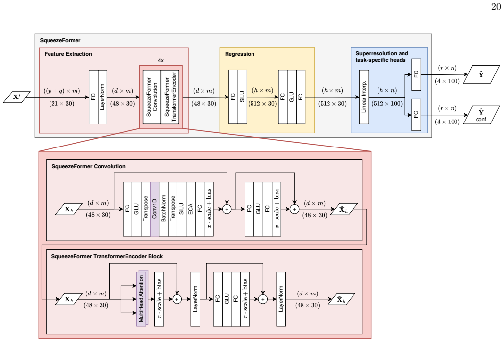
Training procedure The Squeezeformer is trained to minimize a two-part loss function comprising a regression loss and a con- fidence loss that serves as regularization [23]. Both loss components are based on the root-mean-squared er- ror (RMSE), where the regression loss minimizes the squared error between predicted and reference profiles, ϵi = Yi − ˆYi 2...
[2]

superreso- lution mode

optimizer. Cosine annealing with warm restarts [28] is used to schedule the learning rate during training, and early stopping based on the validation loss is applied to prevent overfitting. C. Baseline models To benchmark the performance of the Squeezeformer, we consider two baseline models that represent the lower and upper performance bounds. The upper ...
[3]

If the ratio of aperture diameter to Fried parameter,D/r 0, is less than one, an optical system operates close to its theoretical op- timum, i.e., is diffraction-limited

Integrated astroclimate parameters Fried ParameterThe Fried parameter [35] (in cen- timeters) is a measure to determine the strength of wave- front distortions caused by OT. If the ratio of aperture diameter to Fried parameter,D/r 0, is less than one, an optical system operates close to its theoretical op- timum, i.e., is diffraction-limited. At the same ...
[4]

Performance metrics Four metrics are used to quantify the performance of the different models in estimating HRC 2 n profiles,r 0, 6 andσ 2 I: bias, centered root-mean-square error (cRMSE), Pearson correlation coefficient (r), and coefficient of de- termination (R2). The bias between an estimated profile variableˆy∈R n and the true profile variabley∈R n is...
[5]

Structure function analysis The structure function (SF) analysis is a method for assessing how well models capture the vertical variability ofC 2 n profiles across different vertical scales [36]. The structure function of a signal is related to its power spec- trum obtained through the Fourier transform [36, 37], so one can loosely think of SF analysis as...
[6]

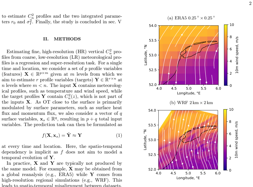
17km×17km at 52 ◦N in the Netherlands) ERA5 reanalysis dataset [18]

and the lower-resolution (0.25◦ ×0.25 ◦ correspond- ing to ca. 17km×17km at 52 ◦N in the Netherlands) ERA5 reanalysis dataset [18]. The WRF data not only have higher horizontal resolution but also higher vertical resolution, with 100 vertical levels between the surface and ca. 20km height, compared to 37 pressure levels in ERA5 up to ca. 30km height. The ...
[7]

TheWRFconfigurationisbasedonPierzynaet al

is used to generate a statistically representative[38], high-resolution training dataset ofC 2 n over the Nether- lands. TheWRFconfigurationisbasedonPierzynaet al
[8]

The aim is to simulate a full year of hourly output at 2km×2km horizontal resolution and at 100 vertical lev- els, reaching up to ca

whereC 2 n is estimated following the variance-based parameterization of He and Basu [40]. The aim is to simulate a full year of hourly output at 2km×2km horizontal resolution and at 100 vertical lev- els, reaching up to ca. 20km in height. To keep this task manageable in terms of computational costs and stor- age requirements, we employ two tricks. First...

2017
[9]

J. W. Hardy,Adaptive Optics for Astronomical Tele- scopes, Oxford Series in Optical and Imaging Sciences, Vol. 16 (Oxford University Press, USA, New York, NY, USA, 1998)

1998
[10]

M. G. Miller and P. L. Zieske,Turbulence Environment Characterization, Technical Report RADC-TR-M9131 (Rome Air Development Center, 1979)

1979
[11]

R. E. Hufnagel, inThe Infrared Handbook(USGPO, Washington, D.C., 1974) 1st ed., p. Chap. 6

1974
[12]

G. C. Valley, Applied Optics19, 574 (1980)

1980
[13]

Ulrich,Hufnagel-Valley Profiles for Specified Values of the Coherence Length and Isoplanatic Angle, Tech

PB. Ulrich,Hufnagel-Valley Profiles for Specified Values of the Coherence Length and Isoplanatic Angle, Tech. Rep. MA-TN-88-013 (W. J. Schafer Associates, 1988)

1988
[14]

R. E. Good, R. R. Beland, E. A. Murphy, J. H. Brown, and E. M. Dewan, inModeling of the Atmosphere, Vol. 0928 (SPIE, Orlando, FL, United States, 1988) pp. 165– 186

1988
[15]

F. G. Smith, J. S. Accetta, and D. L. Shumaker,At- mospheric Propagation of Radiation, The Infrared & Electro-Optical Systems Handbook, Vol. 2 (Infrared In- formation Analysis Center, 1993)

1993
[16]

Comeron, F

A. Comeron, F. Dios, A. Rodriguez, J. A. Rubio, M. Reyes, and A. Alonso, inOptics & Photonics 2005, edited by D. G. Voelz and J. C. Ricklin (San Diego, Cal- ifornia, USA, 2005) p. 58920O

2005
[17]

L. C. Andrews, R. L. Phillips, D. Wayne, T. Leclerc, P. Sauer, R. Crabbs, and J. Kiriazes, inAtmospheric Propagation VI, Vol. 7324 (SPIE, 2009) pp. 11–22

2009
[18]

L.B.StottsandL.C.Andrews,OpticsExpress31,14265 (2023)

2023
[19]

Dasgupta, C

A. Dasgupta, C. Cicalla, B. Mendoza, and D. Foti, Radio Science61, e2025RS008369 (2026)

2026
[20]

W. C. Skamarock, J. B. Klemp, J. Dudhia, D. O. Gill, Z. Liu, J. Berner, W. Wang, J. G. Powers, M. G. Duda, D. M. Barker, and X.-Y. Huang,A Description of the Advanced Research WRF Model Version 4, Tech. Rep. (UCAR/NCAR, 2021)

2021
[21]

Masciadri, J

E. Masciadri, J. Vernin, and P. Bougeault, Astronomy and Astrophysics Supplement Series137, 185 (1999)

1999
[22]

Cherubini, S

T. Cherubini, S. Businger, R. Lyman, and M. Chun, Journal of Applied Meteorology and Climatology47, 1140 (2008)

2008
[23]

Giordano, J

C. Giordano, J. Vernin, H. Trinquet, and C. Muñoz- Tuñón, Monthly Notices of the Royal Astronomical So- ciety440, 1964 (2014)

1964
[24]

S. Basu, J. Osborn, P. He, and A. W. DeMarco, Monthly Notices of the Royal Astronomical Society497, 2302 (2020)

2020
[25]

Rafalimanana, C

A. Rafalimanana, C. Giordano, A. Ziad, and E. Aristidi, Publications of the Astronomical Society of the Pacific 134, 055002 (2022). 16

2022
[26]

Hersbach, B

H. Hersbach, B. Bell, P. Berrisford, S. Hirahara, A. Horányi, J. Muñoz-Sabater, J. Nicolas, C. Peubey, R. Radu, D. Schepers, A. Simmons, C. Soci, S. Ab- dalla, X. Abellan, G. Balsamo, P. Bechtold, G. Biavati, J. Bidlot, M. Bonavita, G. Chiara, P. Dahlgren, D. Dee, M. Diamantakis, R. Dragani, J. Flemming, R. Forbes, M. Fuentes, A. Geer, L. Haimberger, S. H...

1999
[27]

A. J. Cannon, S. R. Sobie, and T. Q. Murdock, Journal of Climate28, 6938 (2015)

2015
[28]

S. Kim, A. Gholami, A. Shaw, N. Lee, K. Mangalam, J. Malik, M. W. Mahoney, and K. Keutzer, Squeeze- former: An Efficient Transformer for Automatic Speech Recognition (2022), arXiv:2206.00888

work page arXiv 2022
[29]

Henkel, Google - ASL Fingerspelling Recognition, 1st place solution (2023)

C. Henkel, Google - ASL Fingerspelling Recognition, 1st place solution (2023)

2023
[30]

Sohn, Stanford - Ribonanza RNA Folding, 2nd place solution (2024)

H. Sohn, Stanford - Ribonanza RNA Folding, 2nd place solution (2024)

2024
[31]

Ron, LEAP - Atmospheric Physics using AI (Clim- Sim), 1st place solution (2024)

S. Ron, LEAP - Atmospheric Physics using AI (Clim- Sim), 1st place solution (2024)

2024
[32]

R. B. Stull,An Introduction to Boundary Layer Meteo- rology(Kluwer Academic Publishers, Dordrecht, 1988)

1988
[33]

Searching for Activation Functions

P. Ramachandran, B. Zoph, and Q. V. Le, Swish: A Self- Gated Activation Function (2017), arXiv:1710.05941 [cs]

work page internal anchor Pith review arXiv 2017
[34]

Y. N. Dauphin, A. Fan, M. Auli, and D. Grangier, in Proceedings of the 34th International Conference on Ma- chine Learning(PMLR, 2017) pp. 933–941

2017
[35]

Decoupled Weight Decay Regularization

I. Loshchilov and F. Hutter, Decoupled Weight Decay Regularization (2019), arXiv:1711.05101 [cs]

work page internal anchor Pith review Pith/arXiv arXiv 2019
[36]

SGDR: Stochastic Gradient Descent with Warm Restarts

I. Loshchilov and F. Hutter, SGDR: Stochastic Gradient Descent with Warm Restarts (2017), arXiv:1608.03983 [cs]

work page internal anchor Pith review arXiv 2017
[37]

J. C. Wyngaard, Y. Izumi, and S. A. Collins, Journal of the Optical Society of America61, 1646 (1971)

1971
[38]

Dimitrov, R

S. Dimitrov, R. Barrios, B. Matuz, G. Liva, R. Mata- Calvo,andD.Giggenbach,InternationalJournalofSatel- lite Communications and Networking34, 625 (2016)

2016
[39]

Camboulives, M.-T

A.-R. Camboulives, M.-T. Velluet, S. Poulenard, L. Saint-Antonin, and V. Michau, Applied Optics57, 709 (2018)

2018
[40]

Osborn, M

J. Osborn, M. J. Townson, O. J. D. Farley, A. Reeves, and R. M. Calvo, Optics Express29, 6113 (2021)

2021
[41]

Walsh and S

S. Walsh and S. Schediwy, Optics Letters48, 880 (2023)

2023
[42]

L. C. Andrews and R. L. Phillips,Laser Beam Propa- gation through Random Media(SPIE, 1000 20th Street, Bellingham, WA 98227-0010 USA, 2005)

2005
[43]

D. L. Fried, JOSA, Vol. 56, Issue 10, pp. 1372-1379 10.1364/JOSA.56.001372 (1966)

work page doi:10.1364/josa.56.001372 1966
[44]

Lovejoy and D

S. Lovejoy and D. Schertzer, Nonlinear Processes in Geo- physics19, 513 (2012)

2012
[45]

Frisch,Turbulence: The Legacy of A.N

U. Frisch,Turbulence: The Legacy of A.N. Kolmogorov (Cambridge University Press, Cambridge, [Eng.] ; New York, 1995)

1995
[46]

Geographical representative requires more ex- tensive WRF simulations

We refer to temporal representativeness for the Nether- lands here. Geographical representative requires more ex- tensive WRF simulations
[47]

Pierzyna, O

M. Pierzyna, O. Hartogensis, S. Basu, and R. Saathof, Applied Optics63, E107 (2024)

2024
[48]

He and S

P. He and S. Basu, inSPIE Optical Engineering + Ap- plications, edited by A. M. J. van Eijk, C. C. Davis, and S. M. Hammel (San Diego, California, United States,
[49]

Schimanke, M

S. Schimanke, M. Ridal, P. Le Moigne, L. Berggren, P. Undén, R. Randriamampianina, U. Andrea, E. Bazile, A. Bertelsen, P. Brousseau, P. Dahlgren, L. Edvins- son, A. El Said, M. Glinton, S. Hopsch, L. Isaksson, R. Mladek, E. Olsson, A. Verrelle, and Z. Wang, CERRA sub-daily regional reanalysis data for Europe on single levels from 1984 to present (2021)

1984
[50]

H. Baki, S. Basu, and G. Lavidas, Wind Energy Science 10, 1575 (2025)

2025
[51]

G. L. Mellor, Journal of the Atmospheric Sciences30, 1061 (1973)

1973
[52]

G. L. Mellor and T. Yamada, Reviews of Geophysics20, 851 (1982)

1982
[53]

M.NakanishiandH.Niino,Boundary-LayerMeteorology 119, 397 (2006)

2006
[54]

Nakanishi and H

M. Nakanishi and H. Niino, Journal of the Meteorological Society of Japan. Ser. II87, 895 (2009)

2009
[55]

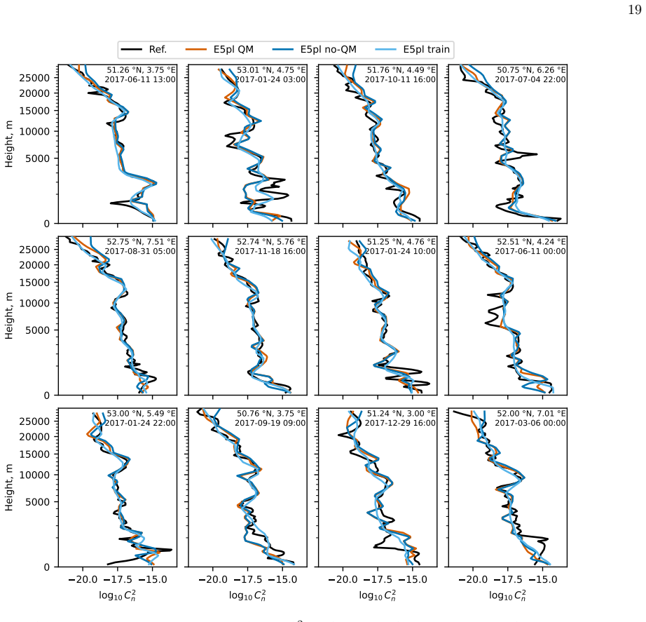
Q.Wang, B.Wu, P.Zhu, P.Li, W.Zuo,andQ.Hu,ECA- Net: Efficient Channel Attention for Deep Convolutional Neural Networks (2020), arXiv:1910.03151 [cs]. Appendix A: Influence of quantile mapping on decoupled training ThisAppendixexaminestheeffectofquantilemapping (QM) on the decoupled training approach by comparing three additional experiments summarized in t...

work page arXiv 2020