arxiv: 2604.11624 · v1 · submitted 2026-04-13 · 🌊 nlin.CD

Recognition: unknown

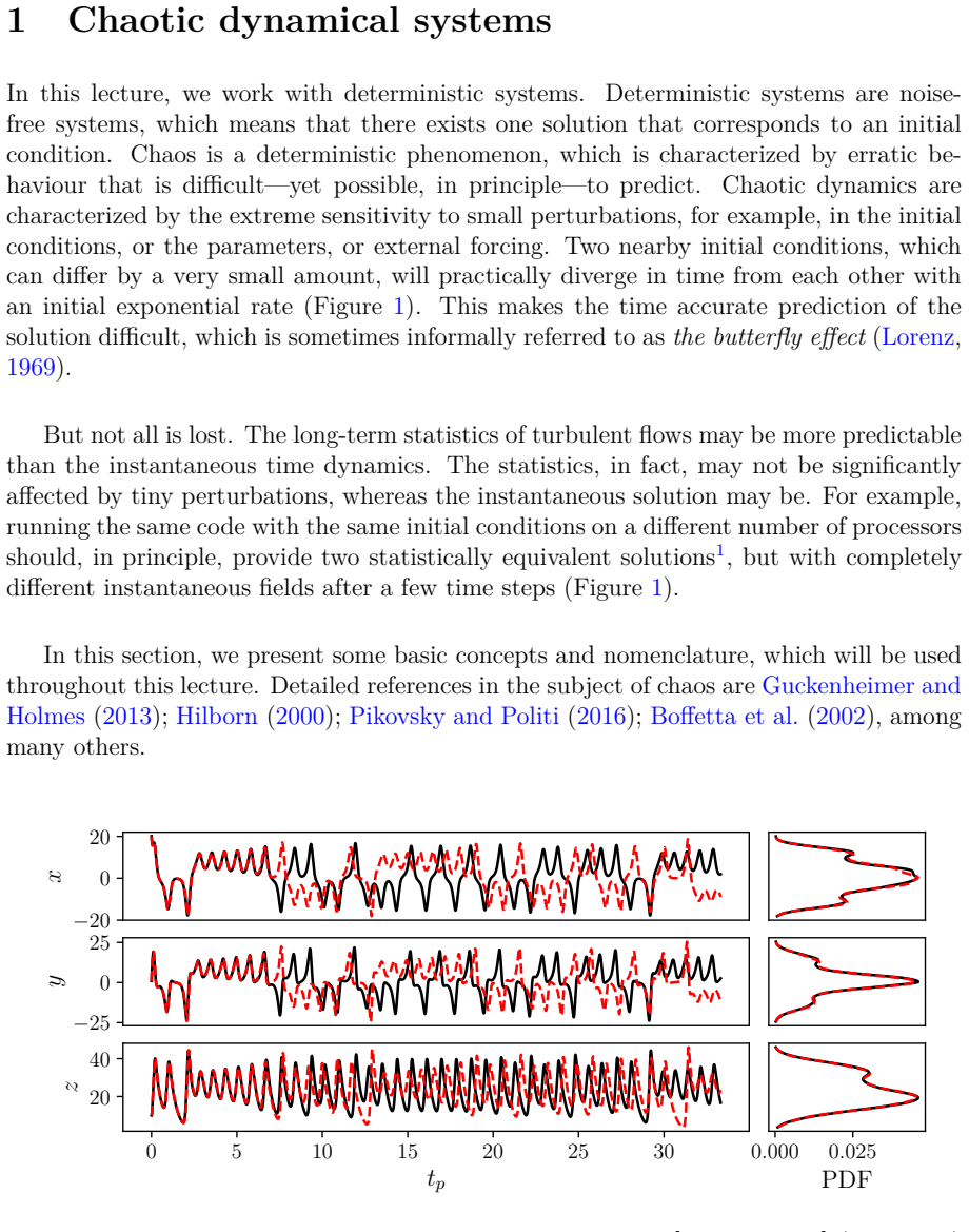
Prediction of chaotic dynamics from data: An introduction

Luca Magri , Andrea N\'ovoa , Elise \"Ozalp

Authors on Pith no claims yet

Pith reviewed 2026-05-10 15:46 UTC · model grok-4.3

classification 🌊 nlin.CD

keywords chaotic dynamicsmachine learningecho state networksLSTM networksLorenz systemtime series forecastingdynamical systemschaos theory

0 comments

The pith

Machine learning can predict chaotic dynamics from finite time series data.

A machine-rendered reading of the paper's core claim, the machinery that carries it, and where it could break.

The paper introduces concepts from dynamical systems and chaos theory to guide the use of machine learning for forecasting chaotic behavior from observed data. It focuses on echo state networks and long short-term memory networks, presenting them with a dynamical systems perspective and illustrating the ideas through examples such as the Lorenz system. A sympathetic reader would care because many real systems display chaotic evolution that is hard to model with traditional equations alone. The chapter also points to online coding tutorials for practical exploration of the methods.

Core claim

This chapter offers a principled approach to the prediction of chaotic systems from data. First, we introduce some concepts from dynamical systems' theory and chaos theory. Second, we introduce machine learning approaches for time-forecasting chaotic dynamics, such as echo state networks and long-short-term memory networks, whilst keeping a dynamical systems' perspective. Third, the lecture contains informal interpretations and pedagogical examples with prototypical chaotic systems (e.g., the Lorenz system).

What carries the argument

Echo state networks and long short-term memory networks, interpreted as recurrent dynamical systems that learn to reproduce chaotic time series from data.

If this is right

Chaotic systems can be forecasted using recurrent neural networks trained on observed time series.
The methods maintain sensitivity to initial conditions and other defining chaotic properties.
Pedagogical examples with the Lorenz system clarify how the machine learning models replicate the dynamics.
Supplementary coding tutorials enable direct implementation and testing of the forecasting techniques.

Where Pith is reading between the lines

These are editorial extensions of the paper, not claims the author makes directly.

The same data-driven perspective could extend to hybrid models that blend learned dynamics with known physical equations for greater robustness.
Statistical long-term behavior rather than exact short-term trajectories may prove more reliable for highly sensitive chaotic systems.
The approach opens questions about how well these networks generalize across different chaotic regimes or parameter ranges.

Load-bearing premise

Finite observed time series data contain sufficient information for the chosen machine learning architectures to capture the essential chaotic dynamics without losing key properties such as sensitivity to initial conditions.

What would settle it

If the trained networks produce time series whose nearby trajectories diverge at a rate inconsistent with the positive Lyapunov exponent of the original system, such as the Lorenz equations, the prediction method would fail to capture the chaotic dynamics.

Figures

Figures reproduced from arXiv: 2604.11624 by Andrea N\'ovoa, Elise \"Ozalp, Luca Magri.

**Figure 2.** Figure 2: Separation trajectory in the Lorenz system over [PITH_FULL_IMAGE:figures/full_fig_p008_2.png] view at source ↗

**Figure 3.** Figure 3: Instantaneous Lyapunov exponents (left) and moving average of the Lyapunov [PITH_FULL_IMAGE:figures/full_fig_p011_3.png] view at source ↗

**Figure 4.** Figure 4: (a) Two long time series for the Lorenz system. (b) Probability density function [PITH_FULL_IMAGE:figures/full_fig_p013_4.png] view at source ↗

**Figure 5.** Figure 5: Different ESN initializations have different optimal hyperparameters ( [PITH_FULL_IMAGE:figures/full_fig_p019_5.png] view at source ↗

**Figure 6.** Figure 6: Typical Echo State Network architectures. Open-loop configuration: Unfolded [PITH_FULL_IMAGE:figures/full_fig_p019_6.png] view at source ↗

**Figure 7.** Figure 7: Split of the input data for the Echo State Network (ESN). During the washout [PITH_FULL_IMAGE:figures/full_fig_p020_7.png] view at source ↗

**Figure 8.** Figure 8: Mean of the Gaussian process reconstruction from a [PITH_FULL_IMAGE:figures/full_fig_p023_8.png] view at source ↗

**Figure 9.** Figure 9: Partition of the data in the different validation strategies ( [PITH_FULL_IMAGE:figures/full_fig_p025_9.png] view at source ↗

**Figure 10.** Figure 10: Schematic representation of the LSTM cell structure. [PITH_FULL_IMAGE:figures/full_fig_p027_10.png] view at source ↗

**Figure 11.** Figure 11: LSTM in open-loop configuration (a) and in closed-loop configuration (b) [PITH_FULL_IMAGE:figures/full_fig_p029_11.png] view at source ↗

**Figure 12.** Figure 12: Illustration of the sliding window technique applied to a trajectory. A fixed [PITH_FULL_IMAGE:figures/full_fig_p030_12.png] view at source ↗

**Figure 13.** Figure 13: Bifurcation diagram for β = 8/3, σ = 10 [PITH_FULL_IMAGE:figures/full_fig_p033_13.png] view at source ↗

**Figure 14.** Figure 14: Strange attractor in the Lorenz system. is λ1 = 0.929. To obtain a better estimate, the calculated value of λ1 should be averaged over many simulations. Tutorial: MagriLab/Tutorials We present a tutorial on the application of LSTM and ESN architectures for modelling the Lorenz 63 system. The Lorenz data is generated using an explicit 4thorder Runge-Kutta method with ∆t = 0.01. For training purposes, we … view at source ↗

**Figure 15.** Figure 15: Closed-loop prediction of LSTM (blue dashed line) and ESN (red dashed line) [PITH_FULL_IMAGE:figures/full_fig_p034_15.png] view at source ↗

**Figure 16.** Figure 16: Attractor of the test data (left), LSTM (middle) and ESN (right). [PITH_FULL_IMAGE:figures/full_fig_p035_16.png] view at source ↗

**Figure 17.** Figure 17: Probability density function (PDF) of the closed-loop prediction of LSTM [PITH_FULL_IMAGE:figures/full_fig_p036_17.png] view at source ↗

read the original abstract

Editorial analysis

A structured set of objections, weighed in public.

Desk editor's note, referee report, simulated authors' rebuttal, and a circularity audit. Tearing a paper down is the easy half of reading it; the pith above is the substance, this is the friction.

Desk Editor's Note private letter to a colleague

This is a clear teaching chapter on applying standard ML tools like echo state networks and LSTMs to forecast chaotic systems, but it contains no new methods, results, or derivations.

read the letter

This chapter is a clear, accessible introduction to using machine learning for short-term prediction of chaotic systems, complete with code examples, but it presents no original research or novel techniques. It does a good job laying out the basics of dynamical systems and chaos theory in simple terms, then showing how echo state networks and LSTMs can be trained on time series from systems like Lorenz to forecast trajectories. The accompanying GitHub tutorials are practical and let readers reproduce the examples easily. That's the strength: it's written for people who want to get their hands dirty with these tools without wading through dense papers. On the downside, everything here is drawn from existing literature. The ML architectures are well-known, the chaotic systems are standard test cases, and the approach doesn't break new ground in either theory or practice. The principled framing is really just keeping the dynamical systems perspective while using off-the-shelf predictors. No new theorems, no comparisons showing superiority, no analysis of long-term behavior or uncertainty. The weakest part is the assumption that the data contains enough info to capture the dynamics without losing sensitivity to initials, but since it's pedagogical, they don't push hard on that. This is for newcomers in engineering or applied science who need a starting point for data-driven chaos prediction. A reader already familiar with reservoir computing or recurrent nets won't find much new. I wouldn't push for peer review on this as a standalone paper. It's better suited as a book chapter or educational note. If the goal is to get the tutorials out there, arXiv is fine as is.

Referee Report

0 major / 3 minor

Summary. The manuscript is an introductory chapter that first reviews key concepts from dynamical systems and chaos theory, then presents machine learning methods for short-term forecasting of chaotic time series (specifically echo state networks and LSTM networks) while maintaining a dynamical-systems viewpoint, illustrates these with pedagogical examples on prototypical attractors such as the Lorenz system, and supplies accompanying reproducible coding tutorials hosted online.

Significance. If the explanations remain accurate and the tutorials execute without modification, the chapter supplies a compact, accessible bridge between nonlinear dynamics and data-driven forecasting techniques. Its explicit emphasis on reproducibility and the dynamical-systems framing of reservoir and recurrent architectures could lower the barrier for researchers entering this intersection, particularly when used in teaching or as a starting reference.

minor comments (3)

[Abstract] The abstract states that the chapter offers 'a principled approach'; because the text is expository and applies previously validated architectures, this phrasing risks overstating novelty. Consider rephrasing to 'a dynamical-systems-guided introduction to ...' or similar in the abstract and opening paragraph.
[Introduction / Tutorial section] The description of the online tutorials is limited to a GitHub link. Adding a brief table or paragraph that lists the specific systems, network hyperparameters, and forecast horizons covered in each notebook would help readers assess coverage before downloading code.
[ML approaches section] Informal interpretations of sensitivity to initial conditions and attractor reconstruction are mentioned; ensure that any statements about preservation of Lyapunov exponents or attractor dimension in the ML forecasts are accompanied by explicit caveats or references to the relevant literature on reservoir computing.

Simulated Author's Rebuttal

0 responses · 0 unresolved

We thank the referee for the positive assessment of the manuscript and the recommendation for minor revision. The referee's summary correctly captures the chapter's structure: an introduction to dynamical systems and chaos concepts, followed by machine-learning approaches (echo state networks and LSTMs) viewed from a dynamical-systems perspective, illustrated with examples such as the Lorenz attractor, and supported by online reproducible tutorials. We are pleased that the significance for lowering the entry barrier in this interdisciplinary area is recognized.

Circularity Check

0 steps flagged

Expository introduction with no load-bearing derivations or self-referential claims

full rationale

The manuscript is explicitly positioned as a pedagogical review that introduces standard dynamical-systems concepts, surveys existing machine-learning architectures (ESNs, LSTMs), and supplies informal examples plus external coding tutorials. No new theorems, parameter fits, uniqueness results, or quantitative predictions are derived; therefore no step reduces by construction to its own inputs, fitted data, or self-citation chains. The text remains self-contained against external benchmarks and contains no circularity.

Axiom & Free-Parameter Ledger

0 free parameters · 1 axioms · 0 invented entities

The chapter rests entirely on standard dynamical systems theory and existing machine learning architectures without introducing new free parameters, ad-hoc axioms, or invented entities.

axioms (1)

standard math Standard concepts from dynamical systems theory and chaos theory hold.
Invoked in the first section to frame the subsequent ML discussion.

pith-pipeline@v0.9.0 · 5389 in / 1055 out tokens · 28599 ms · 2026-05-10T15:46:10.043960+00:00 · methodology

discussion (0)

Reference graph

Works this paper leans on

7 extracted references

[1]

Bennetin, G., Galgani, L., Giorgilli, A., and Strelcyn, J.-M. (1980). Lyapunov character- istic exponents for smooth dynamical systems and for hamiltonian systems: A method for computing all of them.Meccanica, 15(9):27. Birkhoff, G. D. (1931). Proof of the ergodic theorem.Proceedings of the National Academy of Sciences, 17(12):656–660. Blonigan, P. J., Fe...

1980
[2]

Harris, C.R., Millman, K.J., vanderWalt, S.J., Gommers, R., Virtanen, P., Cournapeau, D., Wieser, E., Taylor, J., Berg, S., Smith, N

Springer Science & Business Media. Harris, C.R., Millman, K.J., vanderWalt, S.J., Gommers, R., Virtanen, P., Cournapeau, D., Wieser, E., Taylor, J., Berg, S., Smith, N. J., Kern, R., Picus, M., Hoyer, S., van Kerkwijk, M. H., Brett, M., Haldane, A., del R’ıo, J. F., Wiebe, M., Peterson, P., G’erard-Marchant, P., Sheppard, K., Reddy, T., Weckesser, W., Abb...

2020
[3]

echo state

Hassanaly, M. and Raman, V. (2019). Ensemble-LES analysis of perturbation response of turbulent partially-premixed flames.Proc. Combust. Inst., 37(2):2249–2257. Hilborn, R. C. (2000).Chaos and nonlinear dynamics: an introduction for scientists and engineers. Oxford university press. Hochreiter, S. and Schmidhuber, J. (1997). Long short-term memory.Neural ...

2019
[4]

Lagaris, I

Cambridge university press. Lagaris, I. E., Likas, A., and Fotiadis, D. I. (1998). Artificial neural networks for solving ordinary and partial differential equations.IEEE Trans. Neural Networks, 9(5):987–

1998
[5]

Lorenz, E. N. (1963). Deterministic Nonperiodic Flow.Journal of the Atmospheric Sci- ences, 20(2):130–141. Lorenz, E. N. (1969). Atmospheric predictability as revealed by naturally occurring ana- logues.Journal of the Atmospheric sciences, 26(4):636–646. Lu, Z., Pathak, J., Hunt, B., Girvan, M., Brockett, R., and Ott, E. (2017). Reservoir observers: Model...

1963
[6]

Oseledets, V. I. (1968). A multiplicative ergodic theorem. characteristic lyapunov, ex- ponents of dynamical systems.Trudy Moskovskogo Matematicheskogo Obshchestva, 19:179–210. Özalp, E., Margazoglou, G., and Magri, L. (2023). Physics-informed long short-term memory for forecasting and reconstruction of chaos. InComputational Science – ICCS 2023, pages 38...

1968
[7]

Virtanen, P

Springer Science & Business Media. Virtanen, P. and et al. (2020). SciPy 1.0: Fundamental Algorithms for Scientific Com- puting in Python.Nature Methods, 17:261–272. Vlachas, P., Pathak, J., Hunt, B., Sapsis, T., Girvan, M., Ott, E., and Koumoutsakos, P. (2020). Backpropagation algorithms and reservoir computing in recurrent neural networks for the foreca...

2020