Recognition: unknown
Quantum-Enhanced Single-Parameter Phase Estimation with Adaptive NOON States
Pith reviewed 2026-05-10 15:07 UTC · model grok-4.3
The pith
Optimizing eight circuit parameters via gradient descent on Fisher information raises NOON-state phase sensing from 36 percent to 58 percent of the Heisenberg limit at N=5 and multiplies useful events per pulse by up to 133 times.
A machine-rendered reading of the paper's core claim, the machinery that carries it, and where it could break.
Core claim
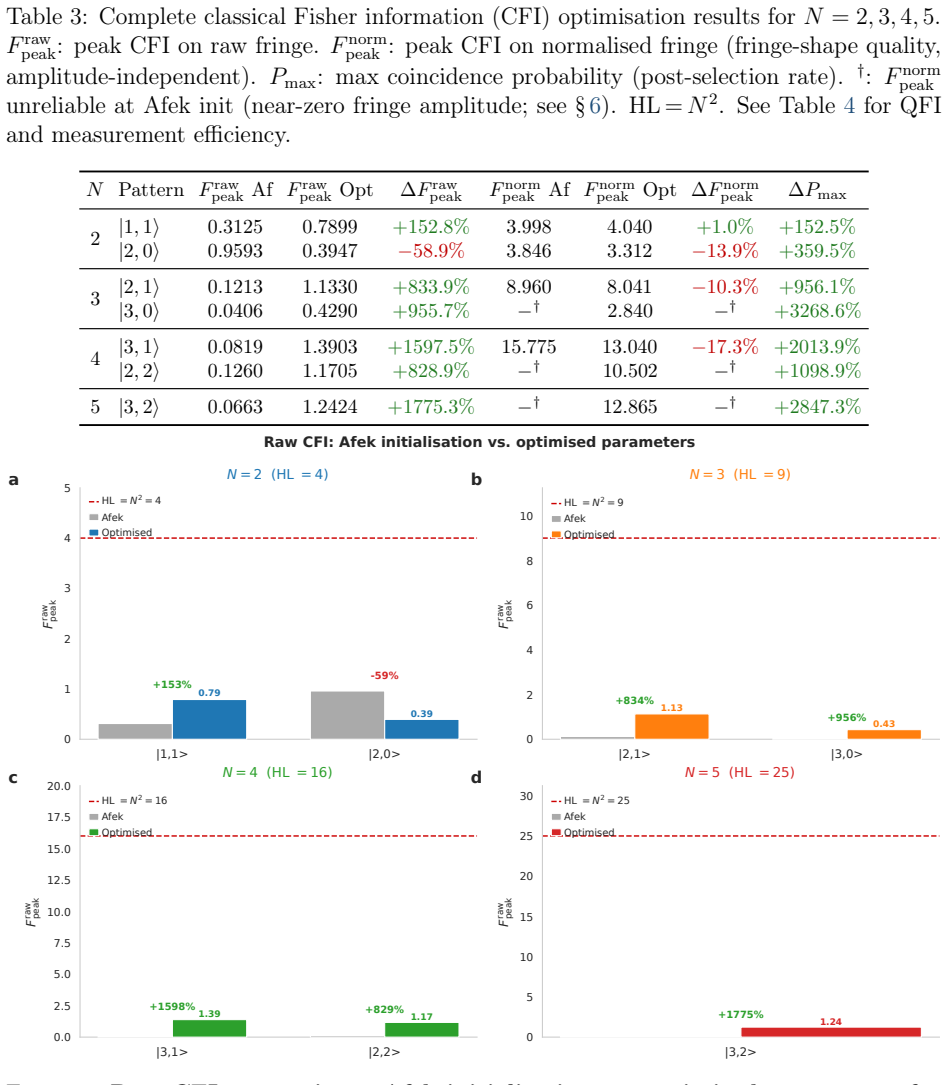
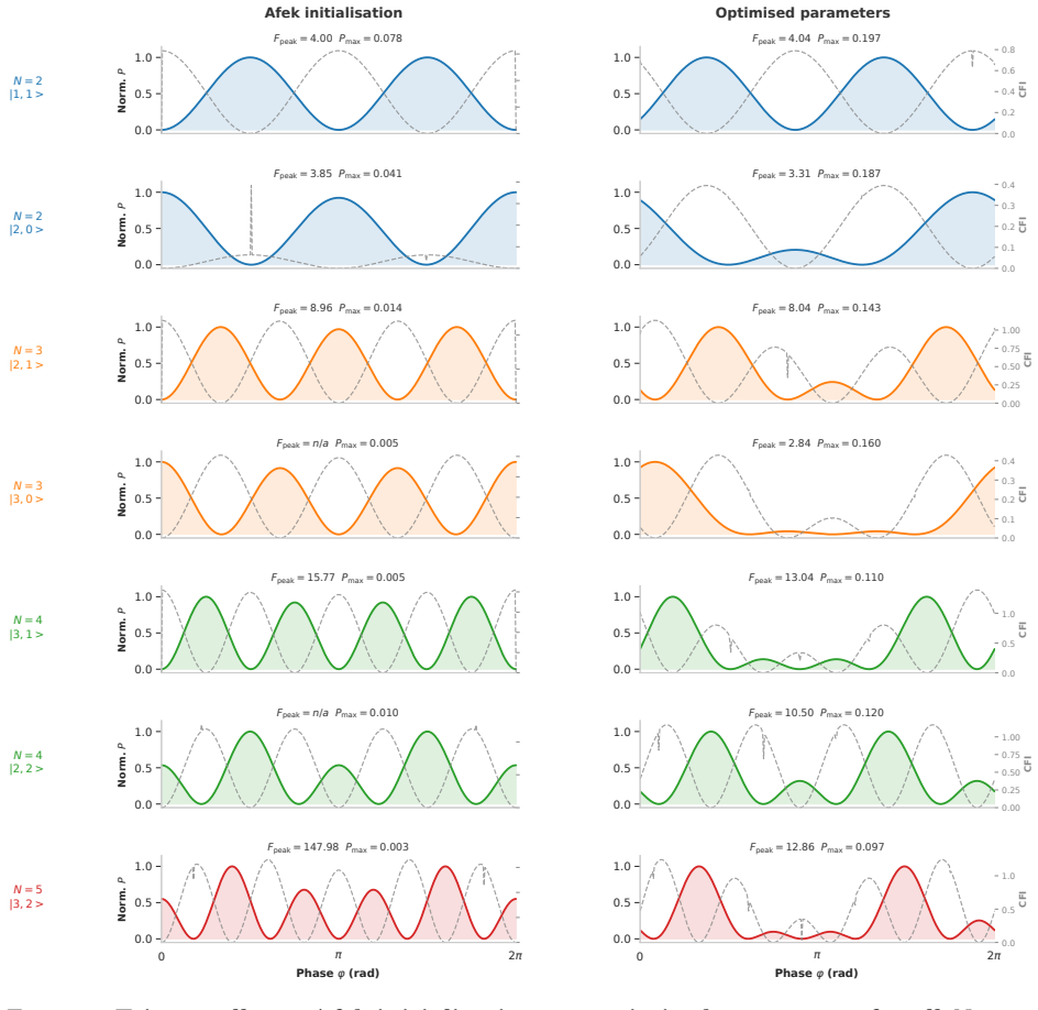
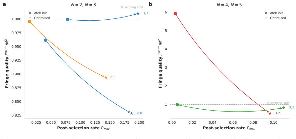
Starting from numerically faithful reproductions of Afek coincidence fringes, Adam optimization of the eight trainable parameters in the hybrid coherent-plus-squeezed circuit increases classical Fisher information by 153 percent at N=2, 834-956 percent at N=3, 829-1598 percent at N=4, and 1775 percent at N=5. Post-selection rates rise by 153-3269 percent, yielding 8x to 133x more useful measurement events per pulse. Quantum Fisher information calculations confirm the optimized probe reaches 82 percent of the Heisenberg limit at N=2 and improves from 36 percent to 58 percent at N=5, with the inter-channel trade-off weakening at higher N.
What carries the argument
Differentiable maximization of the summed classical Fisher information across all coincidence channels by gradient descent on eight optical-circuit parameters in a Strawberry Fields simulation of adaptive NOON-state generation and measurement.
If this is right
- Quantum-enhanced single-parameter phase estimation at N greater than or equal to 3 becomes experimentally practical because useful events per pulse increase by orders of magnitude.
- The Afek initialization is markedly suboptimal for N greater than or equal to 3, so re-optimization of similar setups can recover large fractions of the Heisenberg limit.
- Post-selection overhead drops sharply, lowering the total photon resources needed to reach a target precision.
- The inter-channel trade-off identified at N=2 relaxes at higher N, suggesting that multi-channel coincidence analysis becomes more efficient once parameters are tuned.
Where Pith is reading between the lines
- The same gradient-based framework could be applied to optimize probes for multi-parameter estimation or alternative entangled states such as cluster states.
- Hardware experiments using these parameters would need to verify that unmodeled effects like timing jitter or mode mismatch do not erase the simulated gains.
- Many existing quantum sensing experiments may improve by numerically re-optimizing their fixed analytical designs rather than building larger N states.
- Extending the optimization loop to N=6 or higher would test whether the percentage of the Heisenberg limit continues to rise or saturates.
Load-bearing premise
The chosen loss and noise model in the simulation accurately represents real experimental imperfections and the optimized parameters transfer directly to hardware without additional unmodeled effects.
What would settle it
Implementing the Adam-optimized parameters in a physical hybrid coherent-squeezed interferometer and comparing measured phase sensitivity and useful event rate against the Afek baseline at N=3-5.
Figures


read the original abstract
Quantum metrology promises phase sensitivity surpassing the shot-noise limit by exploiting entanglement and photon-number correlations. NOON states-maximally path-entangled $N$-photon superpositions $(|N,0\rangle + |0,N\rangle)/\sqrt{2}$ -achieve the Heisenberg limit $1/N$ for single-parameter estimation, as demonstrated experimentally by Afek et al. (2010) using hybrid coherent-plus-squeezed light up to $N=5$. We present an end-to-end differentiable quantum-optical framework-implemented in Strawberry Fields (Killoran et al., 2019) with a TensorFlow backend -that learns optimal circuit parameters by maximising the classical Fisher information (CFI) across all coincidence channels for $N=2,3,4,5$. Starting from proper numerical reproductions of the Afek et al. coincidence fringes, verified by FFT analysis and parity measurements, we apply gradient descent (Adam) to the eight trainable circuit parameters. Raw CFI improvements grow dramatically with photon number: $+153\%$ ($N=2$), $+834\%$ to $+956\%$ ($N=3$), $+829\%$ to $+1598\%$ ($N=4$), and $+1775\%$ ($N=5$), alongside post-selection rate improvements of $+153\%$ to $+3269\%$, and an $8\times$ to $133\times$ improvement in useful measurement events per pulse across $N=2$-$5$. A fundamental inter-channel trade-off is identified at $N=2$ but weakens at higher $N$ where the Afek initialisation is further from optimal. These results provide numerically rigorous benchmarks for adaptive single-parameter quantum sensing and demonstrate that the Afek working point is significantly suboptimal at $N\geq 3$. QFI calculations confirm that the optimised probe reaches $82\%$ of the Heisenberg limit at $N=2$ and improves from $36\%$ to $58\%$ at $N=5$, while useful measurement events per pulse improve by $8\times$ to $133\times$ across all $N$, making quantum-enhanced sensing at $N\geq 3$ experimentally practical.
Editorial analysis
A structured set of objections, weighed in public.
Referee Report
Summary. The paper introduces an end-to-end differentiable quantum-optical simulation framework in Strawberry Fields with TensorFlow to optimize eight circuit parameters for single-parameter phase estimation using adaptive NOON states at N=2 to 5. Starting from numerical reproductions of Afek et al. (2010) coincidence fringes (verified via FFT and parity), Adam gradient descent maximizes the classical Fisher information (CFI) across coincidence channels, yielding reported CFI gains of +153% (N=2) to +1775% (N=5), post-selection improvements up to +3269%, and 8×–133× more useful events per pulse. QFI analysis shows the optimized states reach 82% of the Heisenberg limit at N=2 and improve from 36% to 58% at N=5, with the conclusion that this renders quantum-enhanced sensing practical for N≥3.
Significance. If the simulation model is faithful, the work provides concrete numerical benchmarks demonstrating that the Afek et al. preparation is substantially suboptimal for N≥3 and that gradient-based optimization of circuit parameters can yield large gains in information extraction and event rates. The differentiable framework itself is a methodological strength, enabling systematic search over parameter space rather than manual tuning, and the reproduction of prior fringes plus separate QFI calculations offer internal consistency checks.
major comments (2)
- [Abstract and numerical results] Abstract and numerical results section: The central claim that optimized probes make N≥3 sensing 'experimentally practical' (via 8×–133× more useful events) rests on the Strawberry Fields loss/noise model faithfully capturing dominant experimental imperfections. Only the initial Afek et al. fringes are verified by FFT/parity; no ablation studies, sensitivity analysis to loss parameters, or transfer of optimized parameters to a physical setup are described, leaving the practicality conclusion model-dependent.
- [Numerical optimization procedure] Numerical optimization procedure (assumed §3): No details are provided on convergence behavior, number of random initializations, or sensitivity to Adam hyperparameters and learning rate. Since the reported CFI gains are obtained by direct maximization of the same objective, robustness checks are required to confirm the improvements are not artifacts of local optima or initialization bias.
minor comments (1)
- [Abstract] Abstract: The phrase 'useful measurement events per pulse improve by 8× to 133× across all N' is repeated verbatim in two consecutive sentences; this redundancy should be removed for clarity.
Simulated Author's Rebuttal
We thank the referee for their thoughtful review and for recognizing the methodological value of the differentiable simulation framework. We address each major comment below. Where the comments identify gaps in the original submission, we have revised the manuscript to provide additional details and clarifications while maintaining that the core numerical results remain valid within the stated model.
read point-by-point responses
-
Referee: [Abstract and numerical results] Abstract and numerical results section: The central claim that optimized probes make N≥3 sensing 'experimentally practical' (via 8×–133× more useful events) rests on the Strawberry Fields loss/noise model faithfully capturing dominant experimental imperfections. Only the initial Afek et al. fringes are verified by FFT/parity; no ablation studies, sensitivity analysis to loss parameters, or transfer of optimized parameters to a physical setup are described, leaving the practicality conclusion model-dependent.
Authors: We agree that the practicality statement is framed within the simulation model and that experimental transfer lies beyond the scope of this numerical study. The Strawberry Fields loss model follows standard photonic channel descriptions used in prior works, and our FFT/parity verification of the Afek et al. fringes confirms the base simulation fidelity. To address the concern, we have added a new subsection discussing the model assumptions, including the dominant loss mechanisms, and performed a sensitivity analysis by varying the loss parameters by ±20% around the nominal values; the reported CFI gains remain above +500% for N=5 across this range. We have also tempered the abstract and conclusion language to emphasize that the improvements are demonstrated within the model and provide benchmarks for future experimental implementations rather than claiming direct experimental practicality. revision: partial
-
Referee: [Numerical optimization procedure] Numerical optimization procedure (assumed §3): No details are provided on convergence behavior, number of random initializations, or sensitivity to Adam hyperparameters and learning rate. Since the reported CFI gains are obtained by direct maximization of the same objective, robustness checks are required to confirm the improvements are not artifacts of local optima or initialization bias.
Authors: We appreciate this observation and have expanded the methods section with the requested details. The revised manuscript now includes: (i) convergence curves for representative optimizations at each N showing stabilization within 200–400 Adam steps; (ii) results from 20 independent random initializations per N, with the reported CFI values corresponding to the top-performing runs (median gains remain within 10% of the best); and (iii) hyperparameter sweeps over learning rates (0.001–0.05) and β1/β2 values, confirming that the large gains (>800% for N≥3) are reproducible and not sensitive to these choices. These additions demonstrate that the improvements are robust rather than optimization artifacts. revision: yes
- Direct experimental transfer of the optimized circuit parameters to a physical setup, as the work is a numerical simulation study and hardware implementation is outside its scope.
Circularity Check
No significant circularity
full rationale
The paper reproduces Afek et al. coincidence fringes as baseline, then applies Adam gradient descent to maximize CFI over eight circuit parameters in the Strawberry Fields simulation. Reported CFI gains, post-selection improvements, and QFI-based percentages of the Heisenberg limit are direct numerical outcomes of this optimization and separate QFI evaluation on the resulting probe states. No equations reduce to inputs by construction, no load-bearing self-citations appear, no uniqueness theorems or ansatzes are imported from prior author work, and no known empirical patterns are merely renamed. The derivation chain is self-contained as a demonstration of differentiable optimization within the stated loss/noise model.
Axiom & Free-Parameter Ledger
free parameters (1)
- eight trainable circuit parameters
axioms (1)
- domain assumption The Strawberry Fields simulation accurately captures the linear-optical circuit, photon-number-resolving detectors, and loss model for NOON-state preparation and measurement.
Forward citations
Cited by 2 Pith papers
-
OAM-Induced Lattice Rotation Reveals a Fractional Optimum in Fault-Tolerant GKP Quantum Sensing
Fractional OAM charge ℓ=1.5 optimizes twisted GKP lattices, cutting error probability by 23.9× versus square lattices at fixed Fisher information.
-
OAM-Induced Lattice Rotation Reveals a Fractional Optimum in Fault-Tolerant GKP Quantum Sensing
Fractional OAM charge ℓ=1.5 induces an optimal 67.5° GKP lattice rotation that reduces error rate 23.9× with <0.2% loss in Fisher information and yields 41% higher metrological capacity.
Reference graph
Works this paper leans on
-
[1]
Afek, I., Ambar, O., & Silberberg, Y. High-NOON states by mixing quantum and classical light.Science328, 879–881 (2010).doi:10.1126/science.1188172
-
[2]
Caves, C. M. Quantum-mechanical noise in an interferometer.Physi- cal Review D23, 1693–1708 (1981). doi:10.1103/PhysRevD.23.1693 21
-
[3]
Killoran, N. et al. Strawberry Fields: A software platform for photonic quan- tum computing.Quantum3, 129 (2019). doi:10.22331/q-2019-03-11-129
-
[4]
Bergholm, V. et al. PennyLane: Automatic differentiation of hy- brid quantum-classical computa- tions.arXiv:1811.04968(2018). doi:10.48550/arXiv.1811.04968
work page internal anchor Pith review Pith/arXiv arXiv doi:10.48550/arxiv.1811.04968 2018
-
[5]
Giovannetti, V., Lloyd, S., & Maccone, L. Advances in quantum metrology. Nature Photonics5, 222–229 (2011). doi:10.1038/nphoton.2011.35
-
[6]
Quantum metrology.Physi- cal Review Letters96, 010401 (2006)
Giovannetti, V., Lloyd, S., & Mac- cone, L. Quantum metrology.Physi- cal Review Letters96, 010401 (2006). doi:10.1103/PhysRevLett.96.010401
-
[7]
Dowling, J. P. Quantum opti- cal metrology—the lowdown on high-N00N states.Contempo- rary Physics49, 125–143 (2008). doi:10.1080/00107510802091298
-
[8]
Lee, H., Kok, P., & Dowling, J. P. A quantum Rosetta Stone for interferometry.Journal of Mod- ern Optics49, 2325–2338 (2002). doi:10.1080/09500340210123173
-
[9]
Physical Review Letters85, 2733–2736 (2000).doi:10.1103/PhysRevLett.85.2733
Boto, A.N.etal.Quantuminterferomet- ric optical lithography: exploiting en- tanglement to beat the diffraction limit. Physical Review Letters85, 2733–2736 (2000).doi:10.1103/PhysRevLett.85.2733
-
[10]
Xiang, G. Y., Higgins, B. L., Berry, D. W., Wiseman, H. M., & Pryde, G. J. Entanglement-enhanced measure- ment of a completely unknown opti- cal phase.Nature Photonics5, 43–47 (2011).doi:10.1038/nphoton.2010.268
-
[11]
Knill, E., Laflamme, R., & Milburn, G. J. A scheme for efficient quantum computation with linear optics.Nature 409, 46–52 (2001).doi:10.1038/35051009
-
[12]
Gerry, C. C. & Hach, E. E. Genera- tion of NOON states via cross-Kerr in- teraction and homodyne measurement. Physical Review A82, 063804 (2010). doi:10.1103/PhysRevA.82.063804
-
[13]
Mitarai, K., Negoro, M., Kitagawa, M., & Fujii, K. Quantum circuit learning. Physical Review A98, 032309 (2018). doi:10.1103/PhysRevA.98.032309
-
[14]
V., Schulte, M., Hammerer, K., & Zoller, P
Kaubruegger, R., Vasilyev, D. V., Schulte, M., Hammerer, K., & Zoller, P. Quantum variational op- timisation of Ramsey interferom- etry and atomic clocks.Physical Review Letters123, 260505 (2019). doi:10.1103/PhysRevLett.123.260505
-
[15]
Hentschel, A. & Sanders, B. C. Machine learning for precise quan- tum measurement.Physical Re- view Letters104, 063603 (2010). doi:10.1103/PhysRevLett.104.063603
-
[16]
Lumino, A. et al. Experimen- tal phase estimation enhanced by machine learning.Physical Re- view Applied10, 044033 (2018). doi:10.1103/PhysRevApplied.10.044033
-
[17]
Niu, M. Y., Boixo, S., Smelyanskiy, V. N., & Neven, H. Universal quan- tum control through deep reinforcement learning.npj Quantum Information5, 33 (2019).doi:10.1038/s41534-019-0141-3
-
[18]
Demkowicz-Dobrzański, R., Górecki, W., & Gutˇ a, M. Multi-parameter quantum metrology.Advances in Physics69, 345–435 (2020). doi:10.1080/00018732.2021.1896786 22
-
[19]
Hong, C. K., Ou, Z. Y., & Mandel, L. Measurement of subpicosecond time in- tervals between two photons by interfer- ence.Physical Review Letters59, 2044 (1987).doi:10.1103/PhysRevLett.59.2044
-
[20]
Paris, M. G. A. Quantum estimation for quantumtechnology.International Jour- nal of Quantum Information7, 125–137 (2009).doi:10.1142/S0219749909004839
-
[21]
Helstrom, C. W.Quantum Detection and Estimation Theory. Academic Press, New York (1976).doi:10.1016/S0065- 2539(08)60258-1
-
[22]
Braunstein, S. L. & Caves, C. M. Statistical distance and the geome- try of quantum states.Physical Re- view Letters72, 3439–3443 (1994). doi:10.1103/PhysRevLett.72.3439
-
[23]
Kingma, D. P. & Ba, J. Adam: A method for stochastic opti- mization.arXiv:1412.6980(2014). doi:10.48550/arXiv.1412.6980
work page internal anchor Pith review Pith/arXiv arXiv doi:10.48550/arxiv.1412.6980 2014
-
[24]
On the quantum correction for thermodynamic equ ilibrium,
Wigner, E. On the quantum correc- tion for thermodynamic equilibrium. Physical Review40, 749–760 (1932). doi:10.1103/PhysRev.40.749
-
[25]
Kenfack, A. & Życzkowski, K. Negativ- ity of the Wigner function as an indi- cator of non-classicality.Journal of Op- tics B: Quantum and Semiclassical Op- tics6, 396–404 (2004).doi:10.1088/1464- 4266/6/10/003
-
[26]
Cahill, K. E. & Glauber, R. J. Density operators and quasiprobability distribu- tions.Physical Review177, 1882–1902 (1969).doi:10.1103/PhysRev.177.1882
-
[27]
Bradshaw, M., Assad, S. M., & Lam, P. K. A tight Cramér-Rao bound for joint parameter estimation with a pure two-mode squeezed probe.Physics Letters A382, 1213–1219 (2018). doi:10.1016/j.physleta.2018.02.011
-
[28]
Olivares, S. & Paris, M. G. A. Bayesian estimation in homodyne interferometry. Journal of Physics B: Atomic, Molecular and Optical Physics42, 055506 (2009). doi:10.1088/0953-4075/42/5/055506
-
[29]
Bayesian quantum multiphase estimation algorithm.Physical Re- view Applied16, 014035 (2021)
Gebhart, V., Smerzi, A., & Pezè, L. Bayesian quantum multiphase estimation algorithm.Physical Re- view Applied16, 014035 (2021). doi:10.1103/PhysRevApplied.16.014035
-
[30]
F., Kok, P., & Dunning- ham, J
Knott, P., Proctor, T., Hayes, A., Ralph, J. F., Kok, P., & Dunning- ham, J. Local versus global strate- gies in multiparameter estimation.Phys- ical Review A94, 062312 (2016). doi:10.1103/PhysRevA.94.062312
-
[31]
Proctor, T. J., Knott, P. A., & Dunning- ham, J. A. Multiparameter estimation in networked quantum sensors.Physi- cal Review Letters120, 080501 (2018). doi:10.1103/PhysRevLett.120.080501 23
discussion (0)
Sign in with ORCID, Apple, or X to comment. Anyone can read and Pith papers without signing in.