arxiv: 2604.12449 · v1 · submitted 2026-04-14 · 📊 stat.CO

Recognition: unknown

Multi-Object Posterior Computation via Gibbs Sampling

Ba-Ngu Vo, Ba Tuong Vo

Pith reviewed 2026-05-10 14:15 UTC · model grok-4.3

classification 📊 stat.CO

keywords multi-object posteriorGibbs samplingBernoulli random finite setsmulti-object smoothingsuperpositional measurementsposterior inferencelow-SNR performance

0 comments

The pith

The multi-object posterior's conditional distributions are Bernoulli random finite sets with explicit existence probabilities and attribute densities.

A machine-rendered reading of the paper's core claim, the machinery that carries it, and where it could break.

The paper shows how to sample from the full multi-object posterior distribution by constructing a Gibbs sampler whose updates rely on simple, explicitly derivable conditionals. These conditionals turn out to be Bernoulli random finite sets whose existence probabilities and attribute densities can be written in closed form for generic measurement likelihoods. If this holds, full-history posterior inference becomes computationally practical instead of intractable, supporting smoothing algorithms that retain past measurements rather than discarding them as filters do. The approach is demonstrated on superpositional measurements, where it maintains performance in low-signal conditions that defeat detection-based methods. Posterior samples also yield direct statistical summaries of object states and parameters.

Core claim

We establish that the conditional distributions of the multi-object posterior are Bernoulli random finite sets with explicit existence probabilities and attribute densities. These conditionals are straightforward to evaluate and sample from, enabling the construction of an efficient Gibbs sampler with standard convergence guarantees. To demonstrate its versatility, we develop the first multi-scan multi-object smoothing algorithm for superpositional measurements.

What carries the argument

The conditional distributions of the multi-object posterior, shown to be Bernoulli random finite sets whose existence probabilities and attribute densities admit closed-form expressions under generic likelihoods.

Load-bearing premise

The multi-object posterior admits conditional distributions that are Bernoulli random finite sets under a generic measurement likelihood function, allowing explicit forms for existence probabilities and attribute densities.

What would settle it

A concrete measurement likelihood and multi-object model for which the true conditional posterior is not a Bernoulli random finite set or for which the derived existence probability and attribute density fail to match the actual conditional.

Figures

Figures reproduced from arXiv: 2604.12449 by Ba-Ngu Vo, Ba Tuong Vo.

**Figure 2.** Figure 2: Ground truth: Four trajectories, with starting and end points [PITH_FULL_IMAGE:figures/full_fig_p007_2.png] view at source ↗

**Figure 3.** Figure 3: Sample superpositional image observations at times [PITH_FULL_IMAGE:figures/full_fig_p008_3.png] view at source ↗

**Figure 5.** Figure 5: Multi-object trajectory estimate from superpositional-measurement [PITH_FULL_IMAGE:figures/full_fig_p008_5.png] view at source ↗

**Figure 8.** Figure 8: Multi-Object posterior Gibbs sampler: OSPA and OSPA [PITH_FULL_IMAGE:figures/full_fig_p009_8.png] view at source ↗

**Figure 9.** Figure 9: GLMB smoother with a simple detector: OSPA and OSPA [PITH_FULL_IMAGE:figures/full_fig_p009_9.png] view at source ↗

**Figure 10.** Figure 10: Posterior probability that the objects (with labels) [PITH_FULL_IMAGE:figures/full_fig_p010_10.png] view at source ↗

**Figure 11.** Figure 11: Posterior probability that objects (20, 3) and (30, 4) travel at speeds within 0.1m/s of each other. between the speeds, then 1(Et(X0:k)) = 1 L L(Xt)1 max x̸=y∈Xt 1 L({x,y}) L ds(x, y) ≤ η . For L = {(20, 3),(30, 4)}, and η = 0.1m/s, the posterior probability of Et(X0:k) is plotted against t on the interval {1 : k} in [PITH_FULL_IMAGE:figures/full_fig_p010_11.png] view at source ↗

read the original abstract

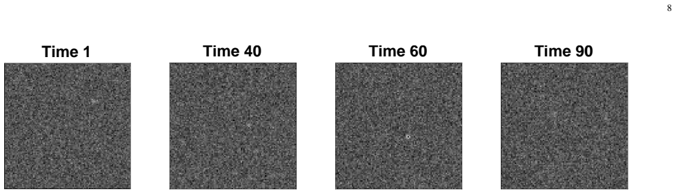
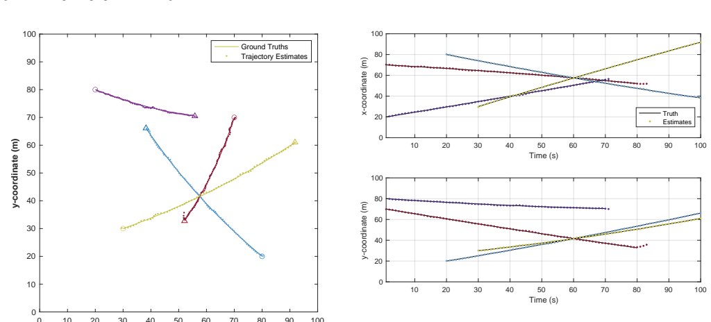
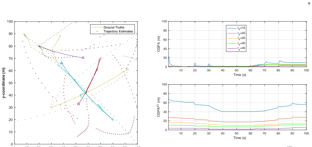
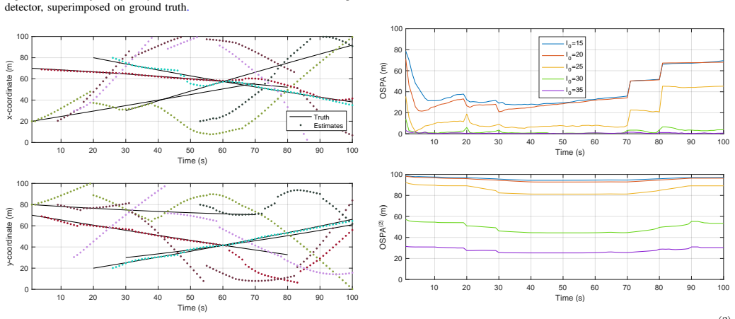
This work presents a tractable approach to multi-object posterior computation under a generic measurement likelihood function. While filtering is a popular solution, valuable historical information is discarded. Posterior inference, which captures the full history of the multi-object states, provides a more comprehensive solution but is notoriously difficult and has received limited attention. Our proposed approach uses Gibbs Sampling (GS) to generate samples from the multi-object posterior. In particular, we establish that the conditional distributions of the multi-object posterior are Bernoulli random finite sets with explicit existence probabilities and attribute densities. These conditionals are straightforward to evaluate and sample from, enabling the construction of an efficient Gibbs sampler with standard convergence guarantees. To demonstrate its versatility, we develop the first multi-scan multi-object smoothing algorithm for superpositional measurements. Numerical experiments show that the proposed method delivers robust performance in challenging low-SNR scenarios where detection based smoothing deteriorates. Moreover, posterior samples obtained from our approach provide statistical characterizations of key variables and parameters, highlighting the advantages of posterior inference. This approach enriches multi-object estimation techniques, which historically lacked smoothing capabilities for non-standard measurements.

Editorial analysis

A structured set of objections, weighed in public.

Desk editor's note, referee report, simulated authors' rebuttal, and a circularity audit. Tearing a paper down is the easy half of reading it; the pith above is the substance, this is the friction.

Desk Editor's Note private letter to a colleague

The paper gives a Gibbs sampler for full multi-object posteriors by turning conditionals into explicit Bernoulli RFS, and claims the first smoothing algorithm for superpositional measurements, but the generic-likelihood claim looks like it may lean on model-specific structure.

read the letter

The core contribution is a Gibbs sampler that samples from the multi-object posterior by showing each full conditional is a Bernoulli random finite set whose existence probability and attribute density can be written down explicitly. They then specialize this to build the first multi-scan smoother for superpositional measurements and report that the resulting samples perform better than detection-based smoothers in low-SNR regimes while also supplying uncertainty measures on the states and parameters.

Referee Report

1 major / 2 minor

Summary. The paper proposes using Gibbs sampling to compute the multi-object posterior under a generic measurement likelihood function p(Z|X). It claims to derive that each full conditional p(X_i | X_{-i}, Z) is exactly a Bernoulli random finite set whose existence probability and attribute density have explicit, closed-form expressions that are straightforward to evaluate and sample from. This enables construction of an efficient Gibbs sampler with standard convergence guarantees. The method is specialized to produce the first multi-scan multi-object smoother for superpositional measurements, with numerical experiments claimed to show robustness in low-SNR regimes where detection-based smoothing fails.

Significance. If the explicit conditional derivations hold without hidden model-specific assumptions, the work would be significant for shifting multi-object estimation from filtering (which discards history) to full posterior inference. It would also extend smoothing to non-standard measurement models. The appeal to standard GS convergence guarantees is a methodological strength, and the provision of posterior samples for statistical characterization of variables is a practical advantage over point-estimate methods.

major comments (1)

[Abstract and derivation of conditionals] Abstract and the section deriving the conditionals: the claim that p(X_i | X_{-i}, Z) is a Bernoulli RFS with explicit existence probability and attribute density for a generic measurement likelihood p(Z|X) is load-bearing for the entire contribution. For non-separable likelihoods (e.g., superpositional Z = sum_j h(X_j) + noise), the conditional density is proportional to the likelihood evaluated on the augmented set times the single-object prior; this expression generally requires an intractable integral over the measurement space for normalization, so neither the existence probability nor direct sampling remains closed-form. The paper's later specialization to superpositional measurements indicates that model-specific cancellations are exploited, but these are not guaranteed for truly generic likelihoods. The derivation must explicitly state the assumptions on p(Z|X) that permit the 'e

minor comments (2)

[Abstract] The abstract refers to 'numerical experiments' demonstrating robust performance but provides no details on simulation setup, SNR values, comparison methods, or quantitative metrics; adding a brief summary or pointer to the relevant table/figure would improve clarity.
[Throughout] Notation for random finite sets and Bernoulli RFS should be introduced with a reference to standard RFS literature on first use to aid readers unfamiliar with the framework.

Simulated Author's Rebuttal

1 responses · 0 unresolved

We thank the referee for their careful reading and constructive feedback. The concern regarding the scope of the conditional derivations and the need to state assumptions on p(Z|X) explicitly is noted. We respond point-by-point below and will revise the manuscript to improve clarity on this load-bearing claim.

read point-by-point responses

Referee: Abstract and the section deriving the conditionals: the claim that p(X_i | X_{-i}, Z) is a Bernoulli RFS with explicit existence probability and attribute density for a generic measurement likelihood p(Z|X) is load-bearing for the entire contribution. For non-separable likelihoods (e.g., superpositional Z = sum_j h(X_j) + noise), the conditional density is proportional to the likelihood evaluated on the augmented set times the single-object prior; this expression generally requires an intractable integral over the measurement space for normalization, so neither the existence probability nor direct sampling remains closed-form. The paper's later specialization to superpositional measurements indicates that model-specific cancellations are exploited, but these are not guaranteed for truly generic likelihoods. The derivation must explicitly state the assumptions on p(Z|X) that permit the 'e

Authors: We agree that the referee correctly identifies a point requiring clarification. The derivation shows that each full conditional is a Bernoulli RFS whose existence probability and attribute density are expressed directly in terms of p(Z|X) evaluated on the augmented set and the single-object prior; this is an explicit functional form without additional model assumptions beyond the standard multi-object Bayesian setup. However, for arbitrary non-separable p(Z|X), the normalizing constant of the attribute density indeed involves an integral that is not guaranteed to be closed-form. In the superpositional case, the additive structure produces cancellations that render the expressions fully closed-form and directly samplable. We will revise the abstract and derivation section to state explicitly that the closed-form property holds when p(Z|X) permits direct pointwise evaluation and the relevant single-object integral is either analytic or numerically tractable (as occurs for the superpositional model). This does not change the core result or the validity of the Gibbs sampler under those conditions, but it accurately bounds the generality claim. revision: yes

Circularity Check

0 steps flagged

No circularity: conditionals derived directly from posterior definition

full rationale

The paper establishes the Bernoulli RFS form of the full conditionals by direct application of the multi-object density definition to p(X_i | X_{-i}, Z), yielding explicit existence probabilities and attribute densities under the stated generic likelihood. This step uses the standard RFS product form and normalization without invoking fitted parameters, self-citations as load-bearing premises, or renaming of known results. The subsequent Gibbs sampler construction follows from these explicit conditionals with standard convergence arguments that are independent of the derivation. No load-bearing step reduces to its own inputs by construction.

Axiom & Free-Parameter Ledger

0 free parameters · 2 axioms · 0 invented entities

The paper relies on random finite set (RFS) modeling which is standard in the domain, and the generic likelihood assumption. No free parameters or new entities mentioned in abstract.

axioms (2)

domain assumption Multi-object states modeled as random finite sets
Standard in the field of multi-object estimation.
domain assumption Measurement likelihood is generic but allows explicit conditional forms
Key to the derivation as per abstract.

pith-pipeline@v0.9.0 · 5481 in / 1224 out tokens · 57449 ms · 2026-05-10T14:15:10.793964+00:00 · methodology

discussion (0)

Reference graph

Works this paper leans on

52 extracted references · 1 canonical work pages

[1]

Bar-Shalom,Multitarget-Multisensor Tracking: Applications and Ad- vances

Y . Bar-Shalom,Multitarget-Multisensor Tracking: Applications and Ad- vances. YBS Publishing, 1998

1998
[2]

S. S. Blackman and R. Popoli,Design and Analysis of Modern Tracking Systems. Artech House, 1999

1999
[3]

Mahler,Advances in Statistical Multisource-Multitarget Information Fusion

R. Mahler,Advances in Statistical Multisource-Multitarget Information Fusion. Artech House, 2014

2014
[4]

An overview of multi- object estimation via labeled random finite set,

B.-N. V o, B.-T. V o, T. D. Nguyen, and C. Shim, “An overview of multi- object estimation via labeled random finite set,”IEEE Trans. Signal Process., 72:4888–4917, 2024

2024
[5]

Past, present, and future of simultaneous localization and mapping: Towards the robust-perception age,

C. Cadena, L. Carlone, H. Carrillo, Y . Latif, D. Scaramuzza, J. Neira, I. D. Reid, and J. J. Leonard, “Past, present, and future of simultaneous localization and mapping: Towards the robust-perception age,”IEEE Transactions on Robotics, vol. 32, no. 6, pp. 1309–1332, 2016

2016
[6]

Maggio and A

E. Maggio and A. Cavallaro,Video Tracking: Theory and Practice. Chichester, UK: Wiley, 2011

2011
[7]

Methods for cell and particle tracking,

E. Meijering, O. Dzyubachyk, and I. Smal, “Methods for cell and particle tracking,”Methods in enzymology, vol. 504, pp. 183–200, 2012

2012
[8]

A survey of data smoothing for linear and nonlinear dynamic systems,

J. Meditch, “A survey of data smoothing for linear and nonlinear dynamic systems,”Automatica, 9(2):151–162, 1973

1973
[9]

Smoothing algorithms for state– space models,

M. Briers, A. Doucet, and S. Maskell, “Smoothing algorithms for state– space models,”Ann. Inst. Statistical Mathematics, 62(1):61–89, 2010

2010
[10]

A tutorial on particle filtering and smooth- ing: Fifteen years later,

A. Doucet and A. Johansen, “A tutorial on particle filtering and smooth- ing: Fifteen years later,”Handbook of Nonlinear Filtering, 12(3):656- 704, 2009

2009
[11]

B. D. Anderson and J. B. Moore,Optimal Filtering. Courier Corpora- tion, 2012

2012
[12]

Särkkä,Bayesian Filtering and Smoothing

S. Särkkä,Bayesian Filtering and Smoothing. Cambridge University Press, 2013

2013
[13]

Goodman, R

I. Goodman, R. Mahler, and H. Nguyen,Mathematics of Data Fusion. Springer Netherlands, 2010

2010
[14]

Labeled random finite sets and multi-object conjugate priors,

B.-T. V o and B.-N. V o, “Labeled random finite sets and multi-object conjugate priors,”IEEE Trans. Signal Process., 61(13):3460–3475, 2013

2013
[15]

Track-before-detect procedures for early detection of moving target from airborne radars,

S. Buzzi, M. Lops, and L. Venturino, “Track-before-detect procedures for early detection of moving target from airborne radars,”IEEE Transactions on Aerospace and Electronic Systems, vol. 41, no. 3, pp. 937–954, 2005

2005
[16]

A comparison of detec- tion performance for several track-before-detect algorithms,

S. J. Davey, M. G. Rutten, and B. Cheung, “A comparison of detec- tion performance for several track-before-detect algorithms,”EURASIP Journal on Advances in Signal Processing, vol. 2008, pp. 1–10, 2007

2008
[17]

A comparative study of track-before-detect algorithms in radar sea clutter,

D. Y . Kim, B. Ristic, X. Wang, L. Rosenberg, J. Williams, and S. Davey, “A comparative study of track-before-detect algorithms in radar sea clutter,” in2019 International Radar Conference (RADAR). IEEE, 2019, pp. 1–6

2019
[18]

Information fusion for industrial mobile platform safety via track-before-detect labeled multi-Bernoulli filter,

T. Rathnayake, R. Tennakoon, A. Khodadadian Gostar, A. Bab- Hadiashar, and R. Hoseinnezhad, “Information fusion for industrial mobile platform safety via track-before-detect labeled multi-Bernoulli filter,”Sensors, vol. 19, no. 9, p. 2016, 2019. 13

2016
[19]

Multi-target Bernoulli track-before-detect for OTHR,

B. Ristic, L. Rosenberg, and D. Y . Kim, “Multi-target Bernoulli track-before-detect for OTHR,”IEEE Transactions on Aerospace and Electronic Systems, 2025. [Online]. Available: https://doi.org/10.1109/TAES.2025.3596188

work page doi:10.1109/taes.2025.3596188 2025
[20]

Multi-frame track-before-detect algorithm for maneuvering target tracking,

W. Yi, Z. Fang, W. Li, R. Hoseinnezhad, and L. Kong, “Multi-frame track-before-detect algorithm for maneuvering target tracking,”IEEE Transactions on Vehicular Technology, vol. 69, no. 4, pp. 4104–4118, 2020

2020
[21]

A particle marginal Metropolis-Hastings multi-target tracker,

T. Vu, B.-N. V o, and R. Evans, “A particle marginal Metropolis-Hastings multi-target tracker,”IEEE Trans. Signal Process., 62(15):3953–3964, 2014

2014
[22]

A multi-scan labeled random finite set model for multi-object state estimation,

B.-N. V o and B.-T. V o, “A multi-scan labeled random finite set model for multi-object state estimation,”IEEE Trans. Signal Process., 67(19):4948–4963, 2019

2019
[23]

Multi-scan multi- sensor multi-object state estimation,

D. Moratuwage, B.-N. V o, B.-T. V o, and C. Shim, “Multi-scan multi- sensor multi-object state estimation,”IEEE Trans. Signal Process., 70:5429–5442, 2022

2022
[24]

An efficient implementation of the generalized labeled multi-Bernoulli filter,

B.-N. V o, B.-T. V o, and H. G. Hoang, “An efficient implementation of the generalized labeled multi-Bernoulli filter,”IEEE Trans. Signal Process., 65(8):1975–1987, 2017

1975
[25]

Linear complexity Gibbs sampling for generalized labeled multi-Bernoulli filtering,

C. Shim, B.-T. V o, B.-N. V o, J. Ong, and D. Moratuwage, “Linear complexity Gibbs sampling for generalized labeled multi-Bernoulli filtering,”IEEE Trans. Signal Process., 71:1981–1994, 2023

1981
[26]

CPHD filters for superpositional sensors,

R. Mahler, “CPHD filters for superpositional sensors,” inSignal Data Process. Small Targets, vol. 7445, 2009, pp. 150–161

2009
[27]

Computationally-tractable approximate PHD and CPHD filters for superpositional sensors,

S. Nannuru, M. Coates, and R. Mahler, “Computationally-tractable approximate PHD and CPHD filters for superpositional sensors,”IEEE J. Sel. Top. Signal Process., vol. 7, no. 3, pp. 410–420, 2013

2013
[28]

A particle multi-target tracker for superpositional measurements using labeled random finite sets,

F. Papi and D. Y . Kim, “A particle multi-target tracker for superpositional measurements using labeled random finite sets,”IEEE Trans. Signal Process., 63(16):4348–4358, 2015

2015
[29]

A robust fast LMB filter for superpositional sensors,

G. Li, P. Wei, Y . Li, L. Gao, and H. Zhang, “A robust fast LMB filter for superpositional sensors,”Signal Process., 174:107606, 2020

2020
[30]

Mahler,Statistical Multisource-Multitarget Information Fusion

R. Mahler,Statistical Multisource-Multitarget Information Fusion. Artech House, 2007

2007
[31]

Multitarget Bayes filtering via first-order multitarget moments,

——, “Multitarget Bayes filtering via first-order multitarget moments,” IEEE Trans. Aerosp. Electron. Syst., 39(4):1152–1178, 2003

2003
[32]

A generalized labeled multi-Bernoulli filter with object spawning,

D. S. Bryant, B.-T. V o, B.-N. V o, and B. A. Jones, “A generalized labeled multi-Bernoulli filter with object spawning,”IEEE Trans. Signal Process., 66(23):6177–6189, 2018

2018
[33]

Tracking cells and their lineages via labeled random finite sets,

T. T. D. Nguyen, B.-N. V o, B.-T. V o, D. Y . Kim, and Y . S. Choi, “Tracking cells and their lineages via labeled random finite sets,”IEEE Trans. Signal Process., 69:5611–5626, 2021

2021
[34]

Interactive multiple-target tracking via labeled multi-Bernoulli filters,

A. K. Gostar, T. Rathnayake, C. Fu, A. Bab-Hadiashar, G. Battistelli, L. Chisci, and R. Hoseinnezhad, “Interactive multiple-target tracking via labeled multi-Bernoulli filters,” inInt. Conf. Control Automat. Inf. Sci., 1–6, 2019

2019
[35]

Annealing Markov chain Monte Carlo with applications to ancestral inference,

C. J. Geyer and E. A. Thompson, “Annealing Markov chain Monte Carlo with applications to ancestral inference,”J. Amer. Statistical Assoc., vol. 90, no. 431, pp. 909–920, 1995

1995
[36]

C. P. Robertet al.,The Bayesian Choice: From Decision-Theoretic Foundations to Computational Implementation. Springer, 2007

2007
[37]

Stochastic relaxation, Gibbs distributions, and the Bayesian restoration of images,

S. Geman and D. Geman, “Stochastic relaxation, Gibbs distributions, and the Bayesian restoration of images,”IEEE Trans. Pattern Anal. Mach. Intell., 6:721–741, 1984

1984
[38]

Markov chains for exploring posterior distributions,

L. Tierney, “Markov chains for exploring posterior distributions,”Annals of Statistics, vol. 22, no. 4, pp. 1701–1762, 1994

1994
[39]

Simple conditions for the geometric convergence of the gibbs sampler,

G. O. Roberts and A. F. M. Smith, “Simple conditions for the geometric convergence of the gibbs sampler,”Stochastic Processes and their Applications, vol. 49, no. 2, pp. 207–216, 1994

1994
[40]

C. P. Robert and G. Casella,Monte Carlo Statistical Methods, 2nd ed. Springer, 2004

2004
[41]

S. P. Meyn and R. L. Tweedie,Markov Chains and Stochastic Stability, 2nd ed. Cambridge University Press, 2009

2009
[42]

J. S. Liu,Monte Carlo Strategies in Scientific Computing. Springer, 2001

2001
[43]

Nonlinear filters with log-homotopy,

F. Daum and J. Huang, “Nonlinear filters with log-homotopy,” inProc. SPIE 6699, Signal and Data Processing of Small Targets 2007, 2007, p. 669918

2007
[44]

On the design of stochastic particle flow filters,

L. Dai and F. Daum, “On the design of stochastic particle flow filters,” IEEE Transactions on Aerospace and Electronic Systems, vol. 59, no. 3, pp. 2439–2450, June 2023

2023
[45]

A consistent metric for performance evaluation of multi-object filters,

D. Schuhmacher, B.-T. V o, and B.-N. V o, “A consistent metric for performance evaluation of multi-object filters,”IEEE Trans. Signal Process., 56(8):3447–3457, 2008

2008
[46]

A solution for large-scale multi- object tracking,

M. Beard, B. T. V o, and B.-N. V o, “A solution for large-scale multi- object tracking,”IEEE Trans. Signal Process., 68:2754–2769, 2020

2020
[47]

An introduction to MCMC for machine learning,

C. Andrieu, N. de Freitas, A. Doucet, and M. I. Jordan, “An introduction to MCMC for machine learning,”Machine Learning, vol. 50, no. 1-2, pp. 5–43, 2003

2003
[48]

An introduction to sequential Monte Carlo methods,

A. Doucet, N. De Freitas, and N. Gordon, “An introduction to sequential Monte Carlo methods,” inSequential Monte Carlo Methods in Pract., 2001, pp. 3–14

2001
[49]

An overview of existing methods and recent advances in sequential Monte Carlo,

O. Cappé, S. J. Godsill, and E. Moulines, “An overview of existing methods and recent advances in sequential Monte Carlo,”IEEE, vol. 95, no. 5, pp. 899–924, 2007

2007
[50]

Sequential Monte Carlo Sam- plers,

P. D. Moral, A. Doucet, and A. Jasra, “Sequential Monte Carlo Sam- plers,”Journal of the Royal Statistical Society: Series B (Statistical Methodology), vol. 68, no. 3, pp. 411–436, 2006

2006
[51]

New theory and numerical results for Gromov’s method for stochastic particle flow filters,

F. Daum, J. Huang, and A. Noushin, “New theory and numerical results for Gromov’s method for stochastic particle flow filters,” in2018 21st International Conference on Information Fusion (FUSION), Cambridge, UK, 2018, pp. 108–115

2018
[52]

Bulletproofing Bayesian particle flow against stiffness,

F. Daum, L. Dai, J. Huang, and A. Noushin, “Bulletproofing Bayesian particle flow against stiffness,” inProc. SPIE 13057, Signal Processing, Sensor/Information Fusion, and Target Recognition XXXIII, 2024, p. 1305708

2024