Recognition: unknown
Causal Graphs for Conditional Parallel Trends
Pith reviewed 2026-05-10 13:51 UTC · model grok-4.3
The pith
Transformed SWIGs let researchers read conditional parallel trends assumptions directly from causal graphs for difference-in-differences designs.
A machine-rendered reading of the paper's core claim, the machinery that carries it, and where it could break.
Core claim
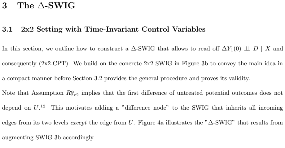
We introduce transformed Single World Intervention Graphs called Δ-SWIGs and prove that d-separation on these graphs identifies the conditional independencies that imply the conditional parallel trends assumption. In multi-period difference-in-differences with time-varying covariates that affect the outcome, valid identification requires controlling for post-treatment values of those covariates. Even with such controls, observed pre-treatment parallel trends only confirm a subset of the assumptions required for unbiased estimates of post-treatment effects.
What carries the argument
The Δ-SWIG, a transformed single-world intervention graph that encodes the differences required to read conditional parallel trends via d-separation.
If this is right
- Applied researchers can check valid conditioning sets for conditional parallel trends by drawing Δ-SWIGs and applying d-separation rules.
- When time-varying covariates influence the outcome, failure to control for their post-treatment values produces identification failure even if pre-treatment trends appear parallel.
- Standard tests for pre-treatment parallel trends alone cannot justify unbiased estimation of post-treatment effects.
- Conditioning strategies that appear sufficient in simple two-period designs may fail in multi-period settings with time-varying covariates.
Where Pith is reading between the lines
- The same graphical approach could be adapted to assess identification in other quasi-experimental designs that rely on trend assumptions.
- Software that automatically constructs Δ-SWIGs from user-specified graphs would lower the barrier to checking conditional parallel trends validity.
- The finding that pre-trend tests are only partially informative suggests re-examining many published difference-in-differences studies that rely solely on such tests for credibility.
Load-bearing premise
The transformation from ordinary causal graphs to Δ-SWIGs preserves exactly the conditional independencies that correspond to the conditional parallel trends assumption holding.
What would settle it
An empirical or simulated example in which d-separation on a Δ-SWIG indicates that a particular conditioning set satisfies conditional parallel trends yet the resulting difference-in-differences estimate remains biased for the causal effect.
Figures
read the original abstract
Difference-in-Differences (DiD) is a widely used research design that often relies on a conditional parallel trends (CPT) assumption. In contrast to settings with unconfoundedness, where causal graphs provide powerful frameworks for reasoning about valid conditioning variables, general-purpose graphical tools for CPT are missing. We introduce transformed Single World Intervention Graphs (SWIGs), the $\Delta$-SWIGs, and prove that they enable us to read off conditional independencies via $d$-separation that imply CPT. Using $\Delta$-SWIGs, we study valid conditioning strategies for DiD in complex settings with multiple periods and time-varying covariates. We show that when time-varying covariates affect the outcome, controlling for post-treatment variables is required for identification. However, even when such controls are included, pre-treatment parallel trends are only informative about a subset of the assumptions required for unbiased post-treatment effects, highlighting the limitations of purely empirical justifications of CPT.
Editorial analysis
A structured set of objections, weighed in public.
Referee Report
Summary. The paper introduces transformed Single World Intervention Graphs (Δ-SWIGs) and proves that d-separation on these graphs identifies conditional independencies implying the conditional parallel trends (CPT) assumption for difference-in-differences (DiD) designs. It applies this framework to multi-period settings with time-varying covariates, demonstrating that post-treatment controls are required when such covariates affect the outcome and that pre-treatment parallel trends only partially inform the assumptions needed for post-treatment effect identification.
Significance. If the Δ-SWIG construction and associated d-separation results hold, the paper supplies the first general-purpose graphical criterion for CPT, analogous to DAG-based tools for unconfoundedness. This would allow systematic derivation of valid conditioning sets in complex DiD applications and provide a formal basis for the paper's caution that empirical pre-treatment checks are insufficient for full CPT justification. The contribution is particularly relevant for applied work involving time-varying covariates.
major comments (2)
- [Definition and properties of Δ-SWIGs] The central claim rests on the Δ-SWIG transformation correctly encoding the causal structure so that d-separation yields exactly the conditional independencies equivalent to CPT. The manuscript must supply an explicit, step-by-step definition of the Δ operator (including its placement relative to post-treatment time-varying covariates and intervention nodes) together with a proof that this mapping preserves potential-outcome independencies without introducing or omitting dependencies in multi-period graphs.
- [Valid conditioning strategies for DiD] The application to multi-period DiD with time-varying covariates concludes that controlling for post-treatment variables is required for identification. This result is load-bearing; the paper should provide a concrete counterexample or derivation showing that failure to condition on post-treatment covariates violates CPT when those covariates affect the outcome, and confirm that the Δ-SWIG d-separation criterion recovers this requirement.
minor comments (2)
- Notation for the Δ operator and the distinction between standard SWIGs and Δ-SWIGs should be introduced with a small illustrative graph before the general theorems.
- The manuscript would benefit from an explicit statement of the maintained assumptions on the underlying causal model (e.g., no unmeasured confounding between treatment and time-varying covariates) that are inherited from the SWIG framework.
Simulated Author's Rebuttal
We thank the referee for their careful reading and constructive comments. We are pleased that the referee sees the potential value of the Δ-SWIG framework for providing a general graphical criterion for conditional parallel trends. We address each major comment below and outline the revisions we will make.
read point-by-point responses
-
Referee: [Definition and properties of Δ-SWIGs] The central claim rests on the Δ-SWIG transformation correctly encoding the causal structure so that d-separation yields exactly the conditional independencies equivalent to CPT. The manuscript must supply an explicit, step-by-step definition of the Δ operator (including its placement relative to post-treatment time-varying covariates and intervention nodes) together with a proof that this mapping preserves potential-outcome independencies without introducing or omitting dependencies in multi-period graphs.
Authors: We agree that greater explicitness will strengthen the exposition. In the revised manuscript we will expand the definition of the Δ operator in Section 2 with a numbered, step-by-step construction that explicitly locates the transformation relative to post-treatment time-varying covariates and intervention nodes. We will also move and enlarge the existing proof (currently in the appendix) to a self-contained subsection that verifies preservation of potential-outcome independencies, with a dedicated multi-period verification showing that no extraneous dependencies are added or omitted. These additions will make the equivalence between Δ-SWIG d-separation and CPT fully transparent. revision: yes
-
Referee: [Valid conditioning strategies for DiD] The application to multi-period DiD with time-varying covariates concludes that controlling for post-treatment variables is required for identification. This result is load-bearing; the paper should provide a concrete counterexample or derivation showing that failure to condition on post-treatment covariates violates CPT when those covariates affect the outcome, and confirm that the Δ-SWIG d-separation criterion recovers this requirement.
Authors: We concur that a concrete illustration will make the load-bearing result more accessible. We will add a simple two-period numerical example (with explicit potential-outcome values) in Section 4 showing that, when a time-varying covariate affects the outcome, omitting its post-treatment realization violates CPT and produces bias. The example will also display the corresponding Δ-SWIG and confirm that d-separation on that graph recovers the necessity of conditioning on the post-treatment covariate. This addition will directly demonstrate both the violation and the criterion's correctness. revision: yes
Circularity Check
No circularity: Δ-SWIGs derived from standard SWIGs and d-separation
full rationale
The paper defines the Δ-SWIG transformation explicitly from existing Single World Intervention Graphs and applies d-separation to derive conditional independencies that imply CPT. No step reduces by construction to a fitted parameter, self-definition, or self-citation load-bearing premise; the central mapping is proved from first principles of graphical causal models rather than assumed or renamed from prior results by the same authors. The contribution is self-contained against external benchmarks such as Richardson-Robins SWIG theory.
Axiom & Free-Parameter Ledger
axioms (2)
- standard math Causal structures are represented by directed acyclic graphs to which SWIGs and d-separation apply.
- domain assumption The Δ-SWIG transformation preserves the conditional independencies relevant to CPT.
invented entities (1)
-
Δ-SWIGs
no independent evidence
Reference graph
Works this paper leans on
-
[1]
Proof.Letmax(g−1, t)≤m≤t ′
Under AssumptionsR α andR Y and consistency we get, for allg, tandt ′ ≥max(g−1, t): ∆Yg−1,t(0)⊥ ⊥X\S g,t |S g,t, Dt′ = 0t′. Proof.Letmax(g−1, t)≤m≤t ′. Define: Sg,t(0m) :=P a G(0m)(Yg−1(0m))\ {U, U Yg−1 , 0m}, P aG(0m)(Yt(0m))\ {U, U Yt , 0m}, By Lemma E.3, withB= X(0m)\S g,t(0m),N= Dt′(0m) we get: ∆Yg−1,t(0m)⊥ ⊥X(0m)\S g,t(0m)|S g,t(0m), Dt′(0m), 41Thos ...
-
[2]
∆Y 1,2(0)⊥ ⊥D2, D3 |X 1, X2, D1 = 0⇒AT T(2,2) is identified;S 2,2(0) =S 2,2 ={X 1, X2}
-
[3]
∆Y 1,3(0)⊥ ⊥D2, D3 |X 1, X3, D1 = 0⇒AT T(2,3) is identified;S 2,3(0) =S 2,3 ={X 1, X3} or applied to SWIG H.1b with treatment-covariate feedback yields
-
[4]
∆Y 1,2(0)⊥ ⊥D2, D3 |X 1, X2(0), D1 = 0⇒AT T(2,2) is identified;S 2,2(0) ={X 1, X2(0)},S 2,2 = {X1, X2}
-
[5]
∆Y 1,3(0)⊥ ⊥D2, D3 |X 1, X3(0,0), D 1 = 0⇒AT T(2,3) isnotidentified;S 2,3(0) ={X 1, X3(0,0)}, S2,3 ={X 1, X3} Figure H.1: SWIGs withT= 4 and no covariate dynamics Y0(0,0,0) Y1(0,0,0) Y2(0,0,0) Y3(0,0,0) D1 0 D2(0) 0 D3(0,0)0 X0 X1 X2 X3 U UY0 UY1 UY2 UY3 +α +α +α +α Y0 :=f Y0(U, X0, UY0) =α(U) +g Y0(X0, UY0) Yt(0t) :=α(U) +g Yt(Xt, UYt), t≥1 D1 :=f D1(U, ...
discussion (0)
Sign in with ORCID, Apple, or X to comment. Anyone can read and Pith papers without signing in.