arxiv: 2604.17045 · v1 · submitted 2026-04-18 · 🌌 astro-ph.SR

Recognition: unknown

Potential of Gaia XP Spectra in Red Giant Star Asteroseismology: A Deep-Learning Approach

Rajarshi Barman , Shatanik Bhattacharya , Shravan M. Hanasoge , Siddharth Dhanpal

Authors on Pith no claims yet

Pith reviewed 2026-05-10 06:32 UTC · model grok-4.3

classification 🌌 astro-ph.SR

keywords red giantsasteroseismologyGaia XPdeep learningCNN-LSTMstellar parametersGalactic archaeologyevolutionary states

0 comments

The pith

Deep learning recovers asteroseismic parameters from Gaia XP spectra with moderate-resolution accuracy.

A machine-rendered reading of the paper's core claim, the machinery that carries it, and where it could break.

The paper tests if Gaia’s low-resolution XP spectra can support asteroseismic analysis of red giant stars by training deep learning models on Kepler data. It finds that the models predict the large frequency separation, maximum oscillation frequency, and dipole period spacing at levels comparable to those from LAMOST spectra. This capability matters because it would multiply the number of stars with seismic measurements by orders of magnitude, aiding studies of stellar interiors and the Galaxy’s history. The approach also maps which spectral regions carry the relevant information and distinguishes between red giant branch and clump stars. Overall, it shows low-resolution data suffice for these global seismic inferences.

Core claim

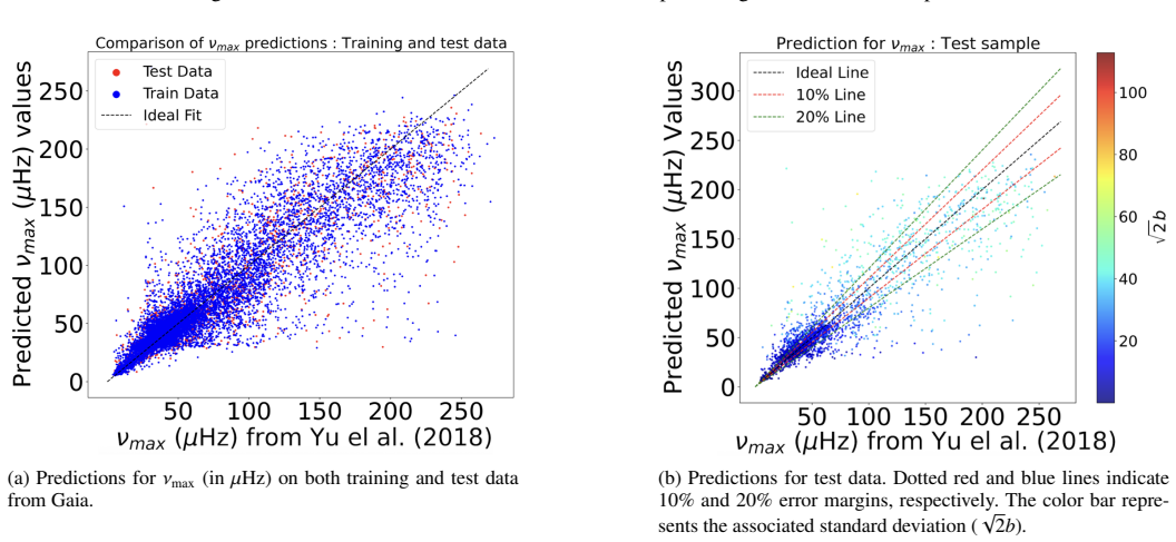
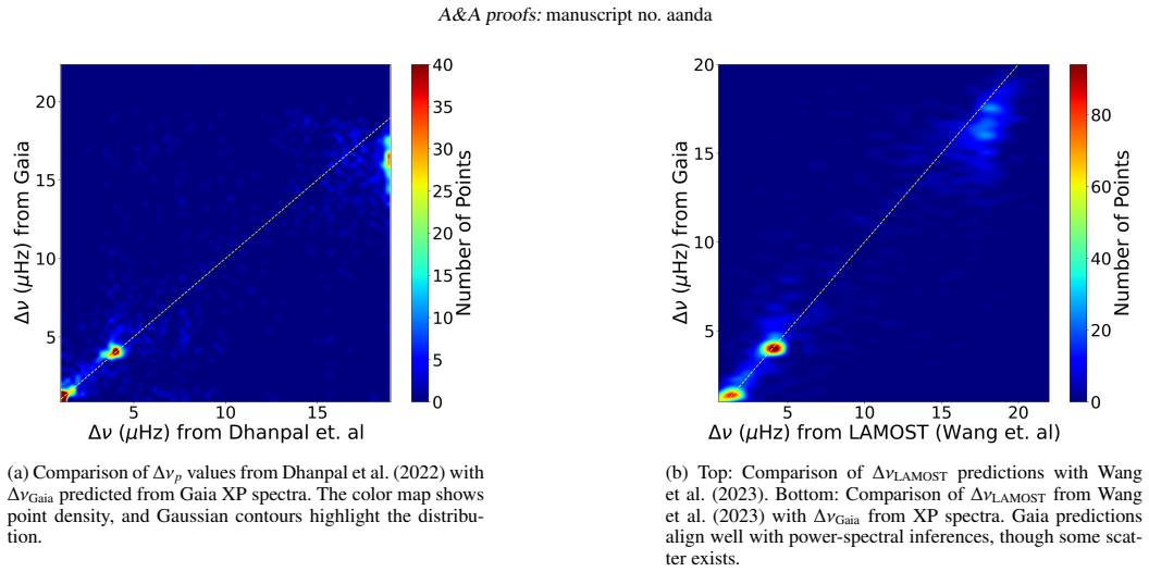
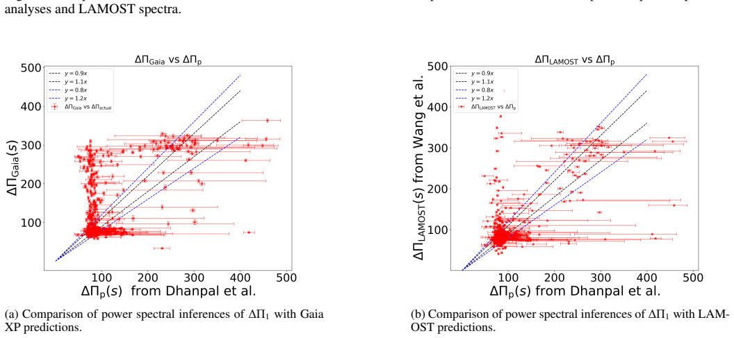
Hybrid CNN-LSTM models trained on red giants with Kepler-derived seismic parameters successfully predict Δν, ν_max, and ΔΠ_1 from Gaia XP spectra, achieving accuracies similar to moderate-resolution spectroscopic surveys and enabling predictions for over 2.5 million stars in Gaia DR3.

What carries the argument

Hybrid CNN-LSTM neural networks that learn subtle spectral signatures correlated with global asteroseismic properties.

If this is right

Seismic parameters can be predicted for more than 2.5 million bright red giants from Gaia DR3.
Population-level asteroseismic studies become feasible on a much larger scale.
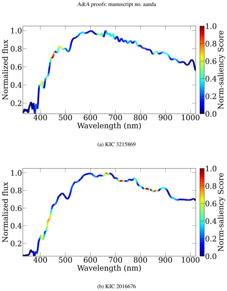
Saliency analysis identifies key wavelength regions linked to seismic parameters.
Distinct spectral behaviors are noted between RGB and RC stars.
A subset of unusual red clump candidates with low Δν is flagged for further study.

Where Pith is reading between the lines

These are editorial extensions of the paper, not claims the author makes directly.

This technique could extend asteroseismology to stars beyond the Kepler field using only Gaia data.
Combining these predictions with Gaia parallaxes and photometry might improve mass and radius estimates across the Galaxy.
Future work could test the models on stars with TESS light curves for validation.
Applying similar methods to other low-resolution spectra might reveal additional evolutionary insights.

Load-bearing premise

The spectral features learned by the models from Kepler stars apply without significant systematic errors to the broader population of red giants observed by Gaia.

What would settle it

A comparison between the deep learning predictions and actual asteroseismic measurements from an independent dataset, such as TESS observations of Gaia red giants, would confirm or refute the claimed accuracy.

Figures

Figures reproduced from arXiv: 2604.17045 by Rajarshi Barman, Shatanik Bhattacharya, Shravan M. Hanasoge, Siddharth Dhanpal.

**Figure 2.** Figure 2: Model (a) :Neural-network architecture used to output ∆ν values. The model takes normalized Gaia XP spectra as input and computes ∆ν and the associated error as defined in the loss function. The CNN layers, LSTM units, and the Dense layers are arranged in sequence as shown. A distinct, independent model with the same architecture is used to predict νmax. Model (b): Model used to infer ∆Π1 from normalized G… view at source ↗

**Figure 3.** Figure 3: Model performance on ∆Π1 prediction [PITH_FULL_IMAGE:figures/full_fig_p006_3.png] view at source ↗

**Figure 4.** Figure 4: The first and second rows show the relative errors in the predicted [PITH_FULL_IMAGE:figures/full_fig_p006_4.png] view at source ↗

**Figure 5.** Figure 5: Performance of the neural network model on predicting [PITH_FULL_IMAGE:figures/full_fig_p007_5.png] view at source ↗

**Figure 6.** Figure 6: Neural network predictions of νmax from Gaia XP spectra. 820–834 nm are particularly noteworthy. As shown in [PITH_FULL_IMAGE:figures/full_fig_p007_6.png] view at source ↗

**Figure 7.** Figure 7: Plots showing log10(∆ν/µHz) and log10(νmax/µHz) inferred by the corresponding trained models from Gaia XP spectra. (Wang et al. 2022; Wang et al. 2023), but at XP resolution, these broad flux-morphology trends become precisely the features that data-driven models capitalize on. For both the ∆ν and ∆Π1 models, we divided the respective parameter ranges into 20 bins and computed the average normalized salie… view at source ↗

**Figure 8.** Figure 8: Saliency maps for the ∆Π1 model, illustrating the spectral regions most relevant for distinguishing red giant branch (RGB) stars from primary and secondary red clump stars (PRCs, SRCs). The curves show the fraction of stars whose normalized saliency scores exceed a threshold of 0.6 at each wavelength bin. While the blue portion of the spectra (≲ 600 nm) shows little distinction between evolutionary states,… view at source ↗

**Figure 9.** Figure 9: Normalized Gaia XP spectra color-coded with saliency scores for a representative RGB star (p [PITH_FULL_IMAGE:figures/full_fig_p010_9.png] view at source ↗

**Figure 10.** Figure 10: Average normalized saliency scores as a function of [PITH_FULL_IMAGE:figures/full_fig_p011_10.png] view at source ↗

**Figure 11.** Figure 11: Average normalized saliency scores as a function of [PITH_FULL_IMAGE:figures/full_fig_p012_11.png] view at source ↗

**Figure 12.** Figure 12: Confusion matrix comparing our ∆ΠGaia-based classification with the evolutionary states reported in the Vrard et al. (2025) catalog for 4311 cross-matched Gaia DR3 red giants. Our method recovers 93% of RC stars and ∼80% of RGB stars, yielding an overall agreement of 84%, demonstrating a good discriminative ability. epoch spectra can be used to derive these parameters using datadriven approaches with … view at source ↗

**Figure 13.** Figure 13: Comparisons of asteroseismic ∆ν values derived from Gaia XP spectra with those from independent power spectrum analyses and LAMOST spectra. (a) Comparison of power spectral inferences of ∆Π1 with Gaia XP predictions. (b) Comparison of power spectral inferences of ∆Π1 with LAMOST predictions [PITH_FULL_IMAGE:figures/full_fig_p014_13.png] view at source ↗

**Figure 14.** Figure 14: Comparison of power spectral inferences of [PITH_FULL_IMAGE:figures/full_fig_p014_14.png] view at source ↗

**Figure 15.** Figure 15: Global asteroseismic parameter distributions derived from Gaia XP spectra. [PITH_FULL_IMAGE:figures/full_fig_p015_15.png] view at source ↗

**Figure 16.** Figure 16: The red circled stars are classified as RCs based on the [PITH_FULL_IMAGE:figures/full_fig_p016_16.png] view at source ↗

**Figure 17.** Figure 17: Example of power spectra of few red giants which have [PITH_FULL_IMAGE:figures/full_fig_p017_17.png] view at source ↗

read the original abstract

Red giants are tracers of stellar evolution & Galactic structure & their asteroseismic properties, particularly large frequency separation, frequency of maximum oscillation power & dipole-mode period spacing, provide direct insight into their internal structure, masses & evolutionary states. Until now, seismic inferences on large stellar samples relied primarily on high-quality light curves from missions such as Kepler & TESS, or on moderate-resolution spectroscopy (LAMOST: R ~ 1800 & APOGEE: R ~ 22500) that clearly preserve information correlated with these seismic quantities. With Gaia XP spectra (R ~ 15-85), the possibility arises to extend asteroseismic measurements to orders of magnitude more stars, despite the much lower spectral res. . Our goal is to assess whether XP spectra retain enough information to enable reliable seismic inference for RGs. We develop hybrid CNN-LSTM models trained on RGs with seismic parameters measured from Kepler photometry. The networks learn the subtle spectral signatures, imprinted through global stellar properties, that correlate with \Delta\nu, \nu_max & \Delta\Pi_1. The models recover all three global asteroseismic parameters from Gaia XP spectra with accuracies comparable to results based on moderate-res. surveys such as LAMOST, demonstrating that even low-res. spectrophotometry carries sufficient information for seismic prediction. Saliency analysis reveals wavelength regions most strongly associated with seismic sensitivity & highlights physically distinct spectral behaviour between RGB & RC stars. Applying our models to Gaia DR3 yields seismic predictions for more than 2.5 M bright RGs, enabling population-level asteroseismic studies on an unprecedented scale. We also identify a small subset of low-\Delta\nu red clump candidates showing unusual spectral-seismic correlations, offering new avenues for investigating evolved stellar populations.

Editorial analysis

A structured set of objections, weighed in public.

Desk editor's note, referee report, simulated authors' rebuttal, and a circularity audit. Tearing a paper down is the easy half of reading it; the pith above is the substance, this is the friction.

Desk Editor's Note private letter to a colleague

Gaia XP spectra can yield asteroseismic predictions for millions of red giants via hybrid CNN-LSTM, but the generalization from Kepler training data needs explicit bias checks to be convincing.

read the letter

The main thing to know is that this paper shows low-resolution Gaia XP spectra contain usable signals for predicting three global asteroseismic parameters in red giants, and they scale the method to produce a catalog for more than 2.5 million stars from Gaia DR3. The hybrid CNN-LSTM model is trained on Kepler seismic labels and then applied forward, with saliency maps added to highlight wavelength regions tied to the predictions and to note differences between RGB and RC stars. They also flag a small set of unusual low-Δν red clump candidates.

Referee Report

3 major / 2 minor

Summary. The paper develops hybrid CNN-LSTM models trained on Kepler red giants with photometric asteroseismic labels to predict the global seismic parameters Δν, ν_max, and ΔΠ1 directly from Gaia XP spectra (R~15-85). It reports that the models achieve accuracies comparable to those obtained from moderate-resolution spectroscopy (e.g., LAMOST), applies the trained networks to >2.5 million Gaia DR3 red giants, performs saliency analysis to identify wavelength regions driving the predictions, and flags a small subset of low-Δν red-clump candidates with anomalous spectral-seismic correlations.

Significance. If the generalization and accuracy claims hold after proper validation, the work would be significant: it shows that low-resolution spectrophotometry encodes sufficient information for asteroseismic inference, enabling population-level studies of stellar masses, ages, and evolutionary states across millions of stars that lack high-quality light curves or moderate-resolution spectra. This would substantially expand the reach of asteroseismology for Galactic archaeology.

major comments (3)

[§4 and §5] §4 (Results) and §5 (Application to Gaia DR3): the central claim that accuracies are 'comparable to LAMOST' is not supported by explicit quantitative metrics (RMSE, MAE, or R²), error distributions, or a clear statement of whether the reported performance is on an independent test set drawn from a different survey or only internal Kepler cross-validation. Without these, the strength of the generalization claim cannot be assessed.
[§3.2] §3.2 (Training and validation procedure): no domain-shift diagnostics are described (e.g., performance stratified by [Fe/H], Teff, or log g; adversarial validation; or comparison of Kepler vs. Gaia parameter distributions). Given the limited metallicity range and selection function of the Kepler training sample, this omission leaves open the possibility of systematic biases when extrapolating to the full Gaia red-giant population.
[§4.3] §4.3 (Saliency maps) and discussion of RGB vs. RC differences: while saliency analysis is presented, it is not accompanied by a quantitative test (e.g., ablation of wavelength regions or comparison against known spectral features) showing that the learned features are physically distinct rather than proxies for Teff/log g/[Fe/H] already encoded in XP spectra.

minor comments (2)

[Abstract and §1] Abstract and §1: abbreviations such as 'res.' and 'M' (for million) should be spelled out on first use for clarity.
[§5] Figure captions and §5: the number of stars in the final Gaia DR3 application sample should be stated precisely (e.g., '2.5 million' rather than '2.5 M') and any quality cuts applied should be listed.

Simulated Author's Rebuttal

3 responses · 0 unresolved

We thank the referee for their thorough and constructive review, which has helped us improve the clarity and rigor of the manuscript. We address each major comment below and have revised the paper accordingly to strengthen the presentation of results and validation procedures.

read point-by-point responses

Referee: [§4 and §5] §4 (Results) and §5 (Application to Gaia DR3): the central claim that accuracies are 'comparable to LAMOST' is not supported by explicit quantitative metrics (RMSE, MAE, or R²), error distributions, or a clear statement of whether the reported performance is on an independent test set drawn from a different survey or only internal Kepler cross-validation. Without these, the strength of the generalization claim cannot be assessed.

Authors: We agree that the original manuscript relied on a qualitative reference to published LAMOST accuracies without direct numerical side-by-side metrics. In the revised version we have added Table 3 in §4, which reports RMSE, MAE, and R² values for our CNN-LSTM models on the held-out Kepler test set together with the corresponding figures quoted from the LAMOST literature for comparable red-giant samples. We have also included residual histograms (new Fig. 4) to display the full error distributions. The performance numbers are obtained from a single 20 % independent hold-out test set drawn from the Kepler training sample (not k-fold cross-validation), and this is now stated explicitly in §3.2 and §4. These additions make the comparability claim quantitatively verifiable. revision: yes
Referee: [§3.2] §3.2 (Training and validation procedure): no domain-shift diagnostics are described (e.g., performance stratified by [Fe/H], Teff, or log g; adversarial validation; or comparison of Kepler vs. Gaia parameter distributions). Given the limited metallicity range and selection function of the Kepler training sample, this omission leaves open the possibility of systematic biases when extrapolating to the full Gaia red-giant population.

Authors: We acknowledge the referee’s concern regarding potential domain shift. The Kepler training set indeed spans a narrower metallicity range than the full Gaia DR3 red-giant population. In the revision we have expanded §3.2 with a new paragraph and accompanying Table 2 that stratifies test-set performance by Teff and log g bins, demonstrating that RMSE remains stable across the parameter space covered by the training data. We have also added Fig. 2, which overlays the [Fe/H], Teff, and log g distributions of the Kepler training sample against the Gaia DR3 application sample. While we did not conduct adversarial validation (which would require additional computational resources beyond the scope of the present study), the stratification and distributional comparison provide a first-order check on extrapolation risk; we now discuss the remaining limitations explicitly in the final section. revision: partial
Referee: [§4.3] §4.3 (Saliency maps) and discussion of RGB vs. RC differences: while saliency analysis is presented, it is not accompanied by a quantitative test (e.g., ablation of wavelength regions or comparison against known spectral features) showing that the learned features are physically distinct rather than proxies for Teff/log g/[Fe/H] already encoded in XP spectra.

Authors: We concur that a purely visual saliency analysis leaves open the possibility that the network is merely recovering already-known stellar-parameter information. In the revised §4.3 we have added a quantitative ablation experiment: we mask the highest-saliency wavelength intervals (identified separately for RGB and RC subsamples) and retrain the models, showing a statistically significant increase in RMSE that exceeds the degradation obtained when masking regions of comparable width but lower saliency. We further compare the locations of the saliency peaks with known atomic and molecular features reported in higher-resolution spectroscopic studies of red giants. These additions demonstrate that the network exploits physically distinct spectral information beyond simple Teff/log g/[Fe/H] proxies. revision: yes

Circularity Check

0 steps flagged

No significant circularity; supervised learning pipeline is self-contained

full rationale

The paper trains hybrid CNN-LSTM models on Gaia XP spectra as inputs with independent Kepler photometric asteroseismic labels (Δν, ν_max, ΔΠ1) as targets. Model outputs for new Gaia stars are generated via learned correlations rather than by algebraic reduction to the input spectra or any fitted parameter. No equations, self-citations, or ansatzes are invoked that would make the predictions equivalent to the training inputs by construction. Accuracy comparisons to LAMOST are external benchmarks, and the 2.5 M star catalog is a forward application, not a tautological renaming. The derivation remains non-circular against external seismic labels.

Axiom & Free-Parameter Ledger

1 free parameters · 1 axioms · 0 invented entities

The central claim rests on the domain assumption that low-resolution XP spectra encode information about global stellar properties that correlate with seismic parameters, plus the empirical assumption that a neural network trained on Kepler stars will generalize to Gaia stars.

free parameters (1)

neural network weights and hyperparameters
All CNN-LSTM parameters are fitted to the Kepler training set to learn the spectral-to-seismic mapping.

axioms (1)

domain assumption Gaia XP spectra contain information correlated with asteroseismic parameters through global stellar properties
Invoked as the basis for training the models on Kepler data.

pith-pipeline@v0.9.0 · 5639 in / 1371 out tokens · 64345 ms · 2026-05-10T06:32:51.212358+00:00 · methodology

discussion (0)

Reference graph

Works this paper leans on

83 extracted references · 4 canonical work pages

[1]

, " * write output.state after.block = add.period write newline

ENTRY address archiveprefix author booktitle chapter edition editor howpublished institution eprint journal key month note number organization pages publisher school series title type volume year label extra.label sort.label short.list INTEGERS output.state before.all mid.sentence after.sentence after.block FUNCTION init.state.consts #0 'before.all := #1 ...
[2]

write newline

" write newline "" before.all 'output.state := FUNCTION n.dashify 't := "" t empty not t #1 #1 substring "-" = t #1 #2 substring "--" = not "--" * t #2 global.max substring 't := t #1 #1 substring "-" = "-" * t #2 global.max substring 't := while if t #1 #1 substring * t #2 global.max substring 't := if while FUNCTION word.in bbl.in " " * FUNCTION format....
[3]

1966, in Stellar Evolution, ed.\ R

Baker, N. 1966, in Stellar Evolution, ed.\ R. F. Stein,& A. G. W. Cameron (Plenum, New York) 333

1966
[4]

1988, A&A, 200, 58

Balluch, M. 1988, A&A, 200, 58

1988
[5]

Cox, J. P. 1980, Theory of Stellar Pulsation (Princeton University Press, Princeton) 165

1980
[6]

N.,& Stewart, J

Cox, A. N.,& Stewart, J. N. 1969, Academia Nauk, Scientific Information 15, 1

1969
[7]

1980, Prog

Mizuno H. 1980, Prog. Theor. Phys., 64, 544

1980
[8]

Tscharnuter W. M. 1987, A&A, 188, 55

1987
[9]

1992, in ASP Conf

Terlevich, R. 1992, in ASP Conf. Ser. 31, Relationships between Active Galactic Nuclei and Starburst Galaxies, ed. A. V. Filippenko, 13

1992
[10]

Yorke, H. W. 1980a, A&A, 86, 286
[11]

F., Tytler, D

Zheng, W., Davidsen, A. F., Tytler, D. & Kriss, G. A. 1997, preprint

1997
[12]

Aerts , C., Mathis , S., & Rogers , T. M. 2019, , 57, 35

2019
[13]

2023 a , , 674, A27

Andrae, R., Fouesneau , M., Sordo , R., et al. 2023 a , , 674, A27

2023
[14]

2023 b , The Astrophysical Journal Supplement Series, 267, 8

Andrae, R., Rix, H.-W., & Chandra, V. 2023 b , The Astrophysical Journal Supplement Series, 267, 8

2023
[15]

G., Belokurov , V., et al

Ardern-Arentsen , A., Kane , S. G., Belokurov , V., et al. 2025, , 537, 1984

2025
[16]

& Celisse, A

Arlot, S. & Celisse, A. 2010, Statistics Surveys, 4

2010
[17]

2006, in ESA Special Publication, Vol

Baglin , A., Auvergne , M., Barge , P., et al. 2006, in ESA Special Publication, Vol. 1306, The CoRoT Mission Pre-Launch Status - Stellar Seismology and Planet Finding, ed. M. Fridlund , A. Baglin , J. Lochard , & L. Conroy , 33

2006
[18]

G., Montalban , J., Kallinger , T., et al

Beck , P. G., Montalban , J., Kallinger , T., et al. 2012, , 481, 55

2012
[19]

R., Mosser , B., Huber , D., et al

Bedding , T. R., Mosser , B., Huber , D., et al. 2011, , 471, 608

2011
[20]

J., Dupret , M

Belkacem , K., Goupil , M. J., Dupret , M. A., et al. 2011, , 530, A142

2011
[21]

2012, CoRR, abs/1206.5533 [ 1206.5533 ]

Bengio, Y. 2012, CoRR, abs/1206.5533 [ 1206.5533 ]

work page arXiv 2012
[22]

2025, DL101 Neural Network Outputs and Loss Functions

Berzal, F. 2025, DL101 Neural Network Outputs and Loss Functions

2025
[23]

2022, Monthly Notices of the Royal Astronomical Society, 511, 5032–5041

Bhambra, P., Joachimi, B., & Lahav, O. 2022, Monthly Notices of the Royal Astronomical Society, 511, 5032–5041

2022
[24]

Boggs, P. T. & Rogers, J. E. 1989

1989
[25]

2004, in ESA Special Publication, Vol

Borucki , W., Koch , D., Boss , A., et al. 2004, in ESA Special Publication, Vol. 538, Stellar Structure and Habitable Planet Finding, ed. F. Favata , S. Aigrain , & A. Wilson , 177--182

2004
[26]

J., Koch , D., Basri , G., et al

Borucki , W. J., Koch , D., Basri , G., et al. 2010, Science, 327, 977

2010
[27]

L., Rix, H.-W., et al

Bovy, J., Nidever, D. L., Rix, H.-W., et al. 2014, The Astrophysical Journal, 790, 127

2014
[28]

Browne, M. W. 2000, Journal of Mathematical Psychology, 44, 108

2000
[29]

& Schwarz , C

Buck , T. & Schwarz , C. 2024, arXiv e-prints, arXiv:2410.16081

work page arXiv 2024
[30]

& Lopes , I

Capelo , D. & Lopes , I. 2023, , 953, 165

2023
[31]

1995, Astrophysical Journal Supplement v

Charbonneau, P. 1995, Astrophysical Journal Supplement v. 101, p. 309, 101, 309

1995
[32]

R., van Saders, J

Claytor, Z. R., van Saders, J. L., Llama, J., et al. 2022, The Astrophysical Journal, 927, 219

2022
[33]

2022, The Astrophysical Journal, 928, 188

Dhanpal, S., Benomar, O., Hanasoge, S., et al. 2022, The Astrophysical Journal, 928, 188

2022
[34]

2023, , 674, A33

Gaia Collaboration , Montegriffo , P., Bellazzini , M., et al. 2023, , 674, A33

2023
[35]

& Ghahramani, Z

Gal, Y. & Ghahramani, Z. 2016, Dropout as a Bayesian Approximation: Representing Model Uncertainty in Deep Learning

2016
[36]

2016, Deep Learning (MIT Press), http://www.deeplearningbook.org

Goodfellow, I., Bengio, Y., & Courville, A. 2016, Deep Learning (MIT Press), http://www.deeplearningbook.org

2016
[37]

& Sauval , A

Grevesse , N. & Sauval , A. J. 1998, , 85, 161

1998
[38]

2009, The elements of statistical learning

Hastie, T., Tibshirani, R., Friedman, J., et al. 2009, The elements of statistical learning

2009
[39]

2025, , 980, 90

Hattori , K. 2025, , 980, 90

2025
[40]

2018, , 853, 20

Hawkins , K., Ting , Y.-S., & Walter-Rix , H. 2018, , 853, 20

2018
[41]

L., & Chen , Y.-Q

He , X.-J., Luo , A. L., & Chen , Y.-Q. 2022, , 512, 1710

2022
[42]

Hjorth, L. U. & Nabney, I. T. 2000, Proceedings of the IEEE-INNS-ENNS International Joint Conference on Neural Networks. IJCNN 2000. Neural Computing: New Challenges and Perspectives for the New Millennium, 4, 455

2000
[43]

& Schmidhuber, J

Hochreiter, S. & Schmidhuber, J. 1997, Neural computation, 9, 1735

1997
[44]

2024, , 271, 13

Huang , B., Yuan , H., Xiang , M., et al. 2024, , 271, 13

2024
[45]

2015, On the metallicity gradients of the Galactic disk as revealed by LSS-GAC red clump stars

Huang, Y., Liu, X.-W., Zhang, H.-W., et al. 2015, On the metallicity gradients of the Galactic disk as revealed by LSS-GAC red clump stars

2015
[46]

J., VanderPlas, J

Ivezi \'c , Z ., Connolly, A. J., VanderPlas, J. T., & Gray, A. 2014, Statistics, data mining, and machine learning in astronomy: a practical Python guide for the analysis of survey data, Vol. 1 (Princeton University Press)

2014
[47]

2022, A Comprehensive Survey of Regression Based Loss Functions for Time Series Forecasting

Jadon, A., Patil, A., & Jadon, S. 2022, A Comprehensive Survey of Regression Based Loss Functions for Time Series Forecasting

2022
[48]

2025, Time series saliency maps: explaining models across multiple domains

Kechris, C., Dan, J., & Atienza, D. 2025, Time series saliency maps: explaining models across multiple domains

2025
[49]

2024, , 691, A98

Khalatyan , A., Anders , F., Chiappini , C., et al. 2024, , 691, A98

2024
[50]

Kingma, D. P. & Ba, J. 2017, Adam: A Method for Stochastic Optimization

2017
[51]

1995, The handbook of brain theory and neural networks, 3361, 1995

LeCun, Y., Bengio, Y., et al. 1995, The handbook of brain theory and neural networks, 3361, 1995

1995
[52]

2022, , 610, 43

Li , G., Deheuvels , S., Ballot , J., & Ligni \`e res , F. 2022, , 610, 43

2022
[53]

Li , J., Wong , K. W. K., Hogg , D. W., Rix , H.-W., & Chandra , V. 2024, , 272, 2

2024
[54]

Lightkurve Collaboration , Cardoso , J. V. d. M., Hedges , C., et al. 2018, Lightkurve: Kepler and TESS time series analysis in Python , Astrophysics Source Code Library

2018
[55]

Liu , C., Bailer-Jones , C. A. L., Sordo , R., et al. 2012, , 426, 2463

2012
[56]

J., Wang , L., Takeda , Y., Bharat Kumar , Y., & Zhao , G

Liu , Y. J., Wang , L., Takeda , Y., Bharat Kumar , Y., & Zhao , G. 2019, , 482, 4155

2019
[57]

L., Smith , G

Martell , S. L., Smith , G. H., & Briley , M. M. 2008, , 136, 2522

2008
[58]

& Gilmore , G

Masseron , T. & Gilmore , G. 2015, , 453, 1855

2015
[59]

& Hawkins , K

Masseron , T. & Hawkins , K. 2017, , 597, L3

2017
[60]

2017, , 464, 3021

Masseron , T., Lagarde , N., Miglio , A., Elsworth , Y., & Gilmore , G. 2017, , 464, 3021

2017
[61]

2013, , 766, 118

Montalb \'a n , J., Miglio , A., Noels , A., et al. 2013, , 766, 118

2013
[62]

2014, , 572, L5

Mosser , B., Benomar , O., Belkacem , K., et al. 2014, , 572, L5

2014
[63]

S., Hochgeschwender, N., & Olivares - M \' e ndez, M

Nair, D. S., Hochgeschwender, N., & Olivares - M \' e ndez, M. A. 2022, CoRR, abs/2202.03870 [ 2202.03870 ]

work page arXiv 2022
[64]

& Hinton, G

Nair, V. & Hinton, G. E. 2010, in Proceedings of the 27th international conference on machine learning (ICML-10), 807--814

2010
[65]

Nix, D. A. & Weigend, A. S. 1994, Proceedings of 1994 IEEE International Conference on Neural Networks (ICNN'94), 1, 55

1994
[66]

M., Ma, X., & Lee, C.-H

Qi, J., Du, J., Siniscalchi, S. M., Ma, X., & Lee, C.-H. 2020, IEEE Signal Processing Letters, 27, 1485

2020
[67]

R., Winn , J

Ricker , G. R., Winn , J. N., Vanderspek , R., et al. 2015, Journal of Astronomical Telescopes, Instruments, and Systems, 1, 014003

2015
[68]

J., Finkbeiner , D

Schlegel , D. J., Finkbeiner , D. P., & Davis , M. 1998, , 500, 525

1998
[69]

Deep Inside Convolutional Networks: Visualising Image Classification Models and Saliency Maps

Simonyan, K., Vedaldi, A., & Zisserman, A. 2013, CoRR, abs/1312.6034

work page Pith review arXiv 2013
[70]

R., Bedding , T

Sreenivas , K. R., Bedding , T. R., Li , Y., et al. 2024, , 530, 3477

2024
[71]

J., Basu, S., Elsworth, Y., & Bedding, T

Stello, D., Chaplin, W. J., Basu, S., Elsworth, Y., & Bedding, T. R. 2009, Monthly Notices of the Royal Astronomical Society: Letters, 400, L80–L84

2009
[72]

2018, , 858, L7

Ting , Y.-S., Hawkins , K., & Rix , H.-W. 2018, , 858, L7

2018
[73]

1989, Nonradial oscillations of stars

Unno , W., Osaki , Y., Ando , H., Saio , H., & Shibahashi , H. 1989, Nonradial oscillations of stars

1989
[74]

E., Rossi , E

Verberne , S., Koposov , S. E., Rossi , E. M., et al. 2024, , 684, A29

2024
[75]

2016, , 588, A87

Vrard , M., Mosser , B., & Samadi , R. 2016, , 588, A87

2016
[76]

2016, Astronomy & Astrophysics, 588, A87

Vrard, M., Mosser, B., & Samadi, R. 2016, Astronomy & Astrophysics, 588, A87

2016
[77]

H., Elsworth , Y., et al

Vrard , M., Pinsonneault , M. H., Elsworth , Y., et al. 2025, , 697, A165

2025
[78]

2022, , 259, 51

Wang , C., Huang , Y., Yuan , H., et al. 2022, , 259, 51

2022
[79]

2023, Astronomy & Astrophysics, 675, A26

Wang, C., Huang, Y., Zhou, Y., & Zhang, H. 2023, Astronomy & Astrophysics, 675, A26

2023
[80]

X., Ness , M., Nordlander , T., et al

Wang , E. X., Ness , M., Nordlander , T., et al. 2025, , 540, 3919

2025

Showing first 80 references.