arxiv: 2604.17835 · v1 · submitted 2026-04-20 · 🌌 astro-ph.HE

Recognition: unknown

Three Subclasses of the Intensity-tracking Pattern in Gamma-Ray Burst Spectral Evolution

Liang Li

Authors on Pith no claims yet

Pith reviewed 2026-05-10 04:38 UTC · model grok-4.3

classification 🌌 astro-ph.HE

keywords gamma-ray burstsspectral evolutionintensity trackingprompt emissionpeak energyFermi observationssingle-pulse GRBs

0 comments

The pith

The intensity-tracking pattern in GRB prompt emission divides into three subclasses by the lag between Ep and flux peaks.

A machine-rendered reading of the paper's core claim, the machinery that carries it, and where it could break.

The paper analyzes a sample of 20 single-pulse gamma-ray bursts from Fermi that display the intensity-tracking spectral evolution. It defines a matched-bin lag between the time of maximum peak energy and maximum flux to classify the bursts. This leads to three types: aligned peaks, Ep peaking first, and flux peaking first. The early Ep peak type is most common and shows unique characteristics in hardness and pulse shape. This classification suggests different underlying radiation mechanisms may be at play in the prompt phase of these bursts.

Core claim

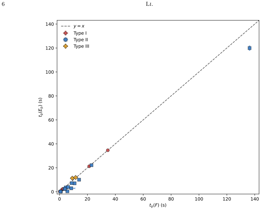
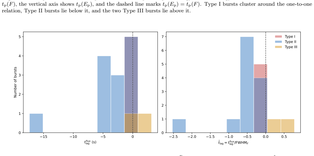
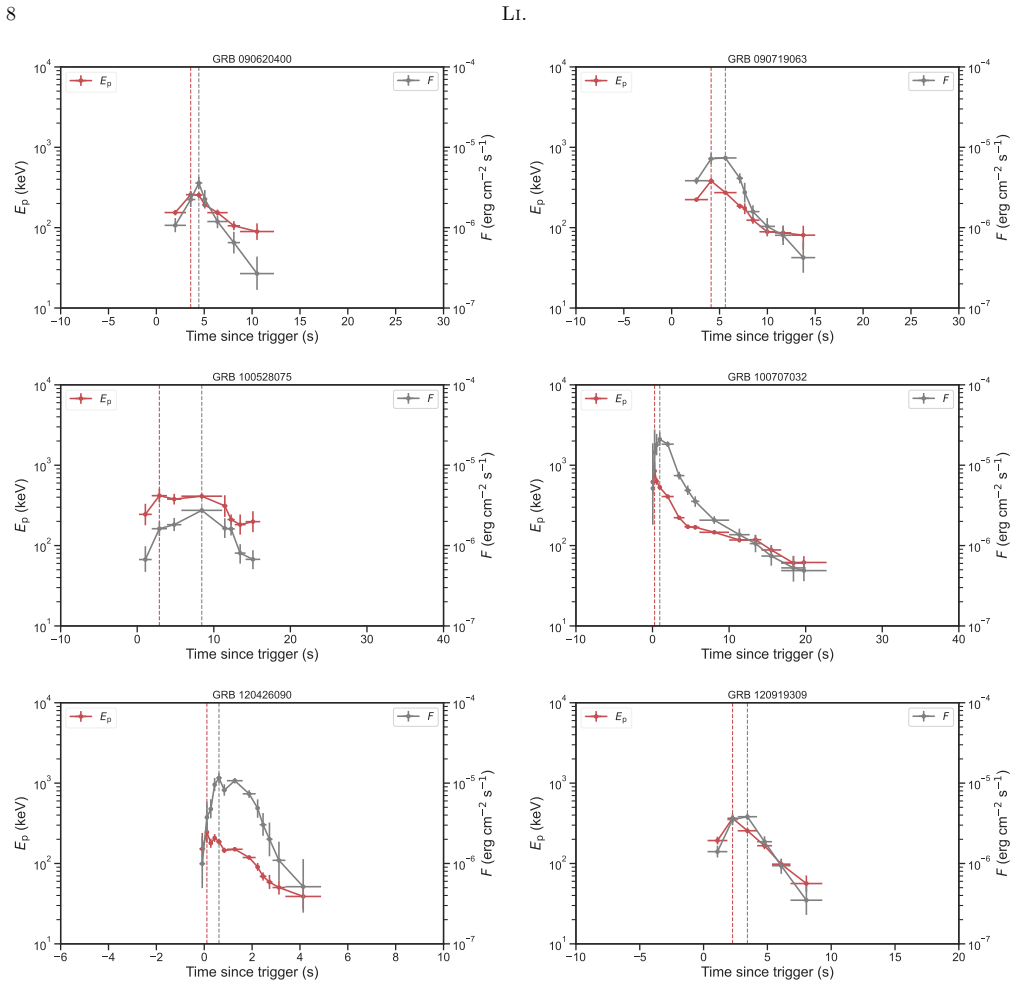
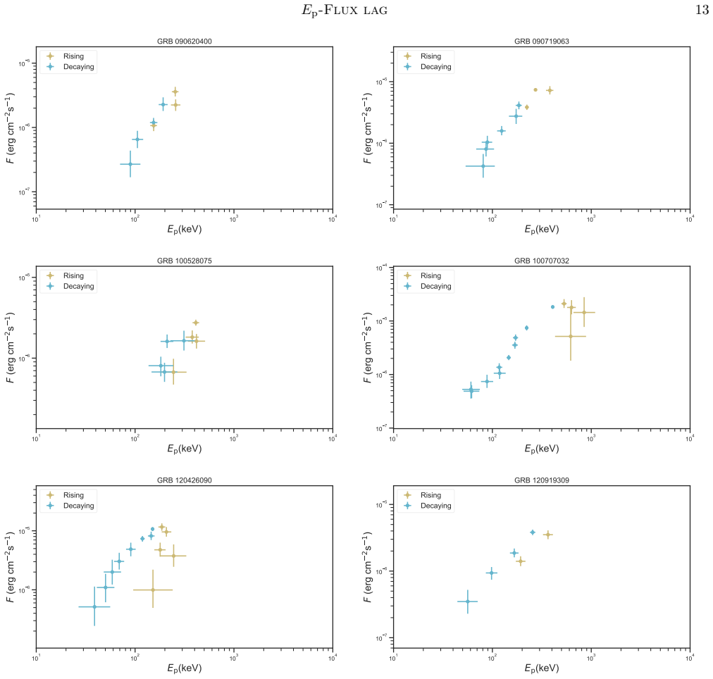
Through time-resolved spectral analysis of 20 single-pulse GRBs showing intensity-tracking, the intensity-tracking pattern is found to subdivide into three distinct subclasses. Type I (5/20) has aligned Ep and flux peaks. Type II (13/20) has Ep peaking before the flux. Type III (2/20) has Ep peaking after the flux. The subclasses differ systematically in spectral hardness, pulse width, and Ep-F branch asymmetry, with Type II being harder and more asymmetric.

What carries the argument

The matched-bin lag t_lag^F, calculated as the difference in peak times of Ep and F using identical time bins from spectral fits, which classifies the subclasses.

If this is right

Type II dominates the sample and is systematically harder than Type I, with broader flux pulses and more asymmetric rising and decaying Ep-F branches.
Type I is consistent with tightly coupled spectral and power evolution.
Type II aligns with nonthermal or hybrid prompt-emission scenarios where spectral hardening precedes peak radiative output.
Type III forms a rare positive-lag tail whose physical origin is uncertain.
These differences indicate that the intensity-tracking pattern is not monolithic but reflects varied physical processes.

Where Pith is reading between the lines

These are editorial extensions of the paper, not claims the author makes directly.

Confirming these subclasses in larger or multi-pulse samples could refine models distinguishing synchrotron from photospheric emission.
Observing whether the lag distribution remains trimodal in different energy bands or detectors would test the robustness of the classification.
Extending the analysis to include polarization or afterglow data might reveal if the subclasses correlate with other GRB properties.

Load-bearing premise

The 20 single-pulse GRBs form a representative sample and the time-resolved spectral analysis with matched bins reliably identifies distinct subclasses free from significant biases or artifacts.

What would settle it

A study of additional single-pulse GRBs showing that the lag values between Ep and F do not separate into three groups around zero lag, or that the reported differences in properties between types disappear with alternative analysis methods.

Figures

Figures reproduced from arXiv: 2604.17835 by Liang Li.

**Figure 1.** Figure 1: Comparison between the peak times of the spectral peak energy and the energy flux. The horizontal axis shows tp(F), the vertical axis shows tp(Ep), and the dashed line marks tp(Ep) = tp(F). Type I bursts cluster around the one-to-one relation, Type II bursts lie below it, and the two Type III bursts lie above it. 15 10 5 0 t flux lag (s) 0 1 2 3 4 5 Number of bursts 2.5 2.0 1.5 1.0 0.5 0.0 0.5 tlag = t flu… view at source ↗

**Figure 2.** Figure 2: Distributions of the peak-time lag. Left: the absolute lag t F lag. Right: the width-normalized lag tˆlag. The earlypeaking Type II events dominate both distributions, while the two Type III bursts form a positive-lag tail [PITH_FULL_IMAGE:figures/full_fig_p006_2.png] view at source ↗

**Figure 3.** Figure 3: All Type I bursts in the sample. In each panel, the red points show Ep(t) and the grey points show F(t) measured from the same time-resolved spectral bins. The peak times are aligned within the timing uncertainty [PITH_FULL_IMAGE:figures/full_fig_p007_3.png] view at source ↗

**Figure 4.** Figure 4: Same as [PITH_FULL_IMAGE:figures/full_fig_p008_4.png] view at source ↗

**Figure 5.** Figure 5: Same as [PITH_FULL_IMAGE:figures/full_fig_p010_5.png] view at source ↗

**Figure 6.** Figure 6: Comparison of the burst-level α summaries for the three subclasses. From left to right, the panels show, the lowenergy photon index at the flux peak, the inverse-variance weighted mean ¯αw, and the hard-bin fraction f−2/3. The scatter points correspond to individual bursts and the box plots mark the overall distribution of each subclass [PITH_FULL_IMAGE:figures/full_fig_p010_6.png] view at source ↗

**Figure 7.** Figure 7: Representative Ep-F relations for selected Type I bursts. In each panel, the time-resolved spectral bins are divided into rising and decaying branches with respect to the flux peak. The two branches largely overlap in the log Ep-log F plane, consistent with the near-aligned peak ordering of this subclass. classes although the small Type III sample precludes a statistically robust characterization of this g… view at source ↗

**Figure 8.** Figure 8: Same as [PITH_FULL_IMAGE:figures/full_fig_p013_8.png] view at source ↗

**Figure 9.** Figure 9: Same as [PITH_FULL_IMAGE:figures/full_fig_p015_9.png] view at source ↗

**Figure 10.** Figure 10: Summary of the branch-dependent Ep-F slopes. Each point represents one burst, with the slope measured on the rising branch plotted against the slope measured on the decaying branch from the relation log Ep = a + b log F. The dashed diagonal marks brise = bdecay. Type I bursts tend to cluster near the diagonal, whereas many Type II bursts lie below it (corresponding to brise < bdecay). The two Type III bur… view at source ↗

**Figure 11.** Figure 11: Flux-pulse morphology by subclass. Left: FWHMF . Right: asymmetry parameter A = (td − tr)/(td + tr). The horizontal bars mark the median value in each subclass. Type II bursts are, on average, broader than Type I bursts, while the Type III sample remains small [PITH_FULL_IMAGE:figures/full_fig_p016_11.png] view at source ↗

**Figure 12.** Figure 12: Distribution of the time-resolved low-energy photon index α for the Type I and Type II bursts. The vertical dashed line marks α = −2/3. Counts are shown without normalization by burst or by bin number. The Type III class is omitted because it contains only two bursts. 10 1 10 2 10 3 10 4 Ep( max)[keV] 2.0 1.5 1.0 0.5 0.0 0.5 1.0 m a x Type I Type II NDP max = 0.5 SCS [PITH_FULL_IMAGE:figures/full_fig_p0… view at source ↗

**Figure 13.** Figure 13: Relation between the maximum low-energy photon index αmax and the corresponding Ep measured in the same time bin for the Type I and Type II bursts. The comparison curves and the horizontal reference line are kept as in the original exploratory figure and are intended only as qualitative guides. The Type III class is omitted because of its small sample size. the spectral peak energy reaches its maximum w… view at source ↗

read the original abstract

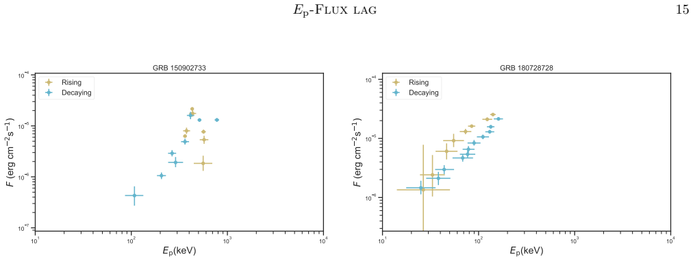
The properties of the spectral evolution during the prompt emission phase of gamma-ray bursts (GRBs), which are closely related to the radiation mechanism (synchrotron or photosphere), are still a subject of debate. Two spectral evolution patterns (``hard-to-soft'' and ``intensity-tracking'') have been commonly observed in GRB prompt emission spectra. Here we present a well-defined sample of 20 single-pulse GRBs detected by \emph{Fermi} whose prompt emission spectra exhibit the intensity-tracking pattern. By performing a time-resolved spectral analysis, we derive $E_{\rm p}$ and the energy flux $F$ from the same time bins and introduce a matched-bin lag, $t_{\rm lag}^{\rm F} \equiv t_{\rm p}(E_{\rm p})-t_{\rm p}(F)$, where $t_{\rm p}$ denotes the time at which each quantity reaches its maximum. We find that the intensity-tracking pattern subdivides into three distinct subclasses: Type I (5/20), with aligned $E_{\rm p}$ and flux peaks; Type II (13/20), with $E_{\rm p}$ peaking before the flux; and Type III (2/20), with $E_{\rm p}$ peaking after the flux. The early-peaking Type~II subclass dominates the sample. The subclasses also exhibit systematic differences in their spectral and temporal properties. Type II bursts are systematically harder than Type I, show broader flux pulses, and more often display asymmetric rising and decaying $E_{\rm p}$-$F$ branches. Type I is consistent with tightly coupled spectral and power evolution, whereas Type II is more naturally explained by nonthermal or hybrid prompt-emission scenarios in which spectral hardening precedes the peak radiative output. Type III appears to form a rare positive-lag tail whose physical origin remains uncertain.

Editorial analysis

A structured set of objections, weighed in public.

Desk editor's note, referee report, simulated authors' rebuttal, and a circularity audit. Tearing a paper down is the easy half of reading it; the pith above is the substance, this is the friction.

Desk Editor's Note private letter to a colleague

The paper splits intensity-tracking GRBs into three lag-based subclasses from a clean 20-event sample, but the distinctions look sensitive to binning and lack uncertainty checks.

read the letter

The main point is that intensity-tracking spectral evolution in single-pulse GRBs divides into three types according to whether the Ep peak aligns with the flux peak, leads it, or lags it. Type II (Ep early) dominates with 13 out of 20 events, while Type I has 5 and Type III only 2. They pull this from Fermi data using time-resolved fits that extract Ep and flux from identical bins, then measure the lag directly as the difference in those peak times. The subclasses show reported differences in hardness, pulse width, and branch asymmetry, which the authors tie to possible differences in radiation physics like nonthermal versus hybrid scenarios. That matched-bin approach is a practical step that sidesteps some of the usual lag-method ambiguities in the literature. The sample selection for single-pulse events is also a reasonable way to reduce complexity. The numbers stay small, especially for the late-peaking class, and the peak assignments come from discrete bins without propagated fit uncertainties or tests against bin-size changes, background choices, or model variations such as Band versus cutoff power-law. A modest shift in a couple of events could alter the counts and the claimed systematic differences. This is aimed at people working on GRB prompt emission mechanisms who already follow spectral evolution studies. It gives them a concrete subdivision and some property contrasts to consider. The work is grounded enough in a defined sample and direct measurements to merit peer review, though referees will likely ask for checks on classification stability.

Referee Report

2 major / 2 minor

Summary. The manuscript analyzes a sample of 20 single-pulse Fermi GRBs exhibiting the intensity-tracking spectral evolution pattern. Using time-resolved spectroscopy to derive Ep and energy flux F from identical time bins, the authors define a matched-bin lag t_lag^F ≡ t_p(Ep) − t_p(F) and classify the bursts into three subclasses: Type I (5/20, aligned peaks), Type II (13/20, Ep peaks before flux), and Type III (2/20, Ep peaks after flux). They report systematic differences in hardness, pulse width, and Ep-F branch asymmetry, interpreting Type I as tightly coupled evolution and Type II as consistent with nonthermal or hybrid emission scenarios.

Significance. If the peak-timing classification proves robust, the work supplies a concrete observational subdivision of the intensity-tracking pattern that could help discriminate among prompt-emission models. The explicit sample size, direct use of matched bins for Ep and F, and reported counts (5/20, 13/20, 2/20) together with noted differences in spectral and temporal properties constitute clear strengths. The dominance of the early-Ep Type II subclass and its association with harder spectra and broader pulses would, if confirmed, provide a useful empirical anchor for theoretical studies of spectral hardening preceding peak radiative output.

major comments (2)

[time-resolved spectral analysis and classification scheme] The subdivision into three subclasses and the reported counts (Type I 5/20, Type II 13/20, Type III 2/20) rest on identification of maxima in the Ep and F light curves. No uncertainties on the peak times t_p(Ep) and t_p(F) are propagated from the time-resolved spectral fits, nor are robustness tests against binning choices, background subtraction, or model variations (Band vs. cutoff power-law) presented. This directly affects the reliability of the lag sign assignments and the claimed systematic differences in hardness, width, and asymmetry.
[sample and subclass statistics] With only 20 events and a strongly dominant Type II bin (13/20), even modest reassignments of a few bursts due to fit or binning variations would alter the reported subclass fractions and the statistical significance of the inter-subclass differences. The manuscript does not quantify how sensitive the classification is to these analysis choices.

minor comments (2)

[sample selection] The abstract states that the sample is 'well-defined' but does not summarize the explicit selection criteria for single-pulse GRBs or for confirming the intensity-tracking pattern; these details should be stated concisely in the main text or a table.
[definition of t_lag^F] Notation for the lag (t_lag^F) and peak times (t_p) is introduced clearly, but the manuscript should specify whether the maxima are determined by simple bin maxima or by any smoothing/interpolation procedure.

Simulated Author's Rebuttal

2 responses · 0 unresolved

We thank the referee for the positive evaluation of our work and the constructive comments on the robustness of the subclassification. We respond point by point to the major comments below.

read point-by-point responses

Referee: [time-resolved spectral analysis and classification scheme] The subdivision into three subclasses and the reported counts (Type I 5/20, Type II 13/20, Type III 2/20) rest on identification of maxima in the Ep and F light curves. No uncertainties on the peak times t_p(Ep) and t_p(F) are propagated from the time-resolved spectral fits, nor are robustness tests against binning choices, background subtraction, or model variations (Band vs. cutoff power-law) presented. This directly affects the reliability of the lag sign assignments and the claimed systematic differences in hardness, width, and asymmetry.

Authors: We agree that propagating uncertainties on the peak times and performing explicit robustness tests would strengthen the analysis. In the revised manuscript we will derive error estimates on t_p(Ep) and t_p(F) from the spectral-fit covariance matrices and conduct additional checks by varying time-binning schemes, background-subtraction methods, and spectral models (Band function versus cutoff power-law). These additions will quantify the stability of the lag assignments and the reported inter-subclass differences. revision: yes
Referee: [sample and subclass statistics] With only 20 events and a strongly dominant Type II bin (13/20), even modest reassignments of a few bursts due to fit or binning variations would alter the reported subclass fractions and the statistical significance of the inter-subclass differences. The manuscript does not quantify how sensitive the classification is to these analysis choices.

Authors: The sample of 20 single-pulse intensity-tracking GRBs is the largest that satisfies our strict selection criteria from the Fermi catalog. In the revision we will add a quantitative sensitivity analysis, for example by perturbing Ep and F values within their fit uncertainties and re-deriving the lag signs, to evaluate the stability of the subclass fractions and the significance of the observed differences in hardness and pulse width. revision: yes

Circularity Check

0 steps flagged

No circularity: classification rests on direct observational peak timing from independent spectral fits

full rationale

The paper selects 20 single-pulse GRBs already identified as showing the intensity-tracking pattern, performs time-resolved spectral fitting to obtain Ep and F in matched bins, defines t_lag^F ≡ t_p(Ep) − t_p(F) as the difference in their observed peak times, and simply counts how many events fall into each sign category (aligned, Ep early, Ep late). This produces an empirical subdivision into three subclasses with reported differences in other properties. No step claims a derivation of one quantity from another that reduces by construction to the input; the lag definition is a measurement convention, not a self-referential equation; no self-citations are invoked as load-bearing uniqueness theorems; and the central result is a count of observed peak alignments rather than a fitted parameter renamed as a prediction. The analysis is therefore self-contained against external benchmarks.

Axiom & Free-Parameter Ledger

0 free parameters · 2 axioms · 0 invented entities

The claim is primarily observational classification; it relies on standard GRB analysis assumptions rather than new free parameters or invented entities.

axioms (2)

domain assumption Single-pulse GRBs can be cleanly isolated from multi-pulse events in the Fermi sample.
Invoked when selecting the 20-burst sample for analysis.
domain assumption Time-resolved spectral fitting yields reliable Ep and flux values whose peak times can be compared directly.
Central to the definition of the matched-bin lag.

pith-pipeline@v0.9.0 · 5632 in / 1323 out tokens · 36670 ms · 2026-05-10T04:38:08.130479+00:00 · methodology

discussion (0)

Reference graph

Works this paper leans on

43 extracted references · 43 canonical work pages

[1]

2018, MNRAS, 475, 1708, doi: 10.1093/mnras/stx3106

Acuner, Z., & Ryde, F. 2018, MNRAS, 475, 1708, doi: 10.1093/mnras/stx3106

work page doi:10.1093/mnras/stx3106 2018
[2]

1993, ApJ, 413, 281, doi: 10.1086/172995

Band, D., Matteson, J., Ford, L., et al. 1993, ApJ, 413, 281, doi: 10.1086/172995

work page doi:10.1086/172995 1993
[3]

Band, D. L. 1997, ApJ, 486, 928, doi: 10.1086/304566

work page doi:10.1086/304566 1997
[4]

N., Fishman, G

Bhat, P. N., Fishman, G. J., Meegan, C. A., et al. 1994, ApJ, 426, 604, doi: 10.1086/174097

work page doi:10.1086/174097 1994
[5]

M., Greiner, J., B´ egu´ e, D., & Berlato, F

Burgess, J. M., Greiner, J., B´ egu´ e, D., & Berlato, F. 2019, MNRAS, 490, 927, doi: 10.1093/mnras/stz2589

work page doi:10.1093/mnras/stz2589 2019
[6]

M., Preece, R

Burgess, J. M., Preece, R. D., Connaughton, V., et al. 2014, ApJ, 784, 17, doi: 10.1088/0004-637X/784/1/17 Caballero-Garc´ ıa, M. D., Gupta, R., Pandey, S. B., et al. 2023, MNRAS, 519, 3201, doi: 10.1093/mnras/stac3629

work page doi:10.1088/0004-637x/784/1/17 2014
[7]

2022, ApJ, 932, 25, doi: 10.3847/1538-4357/ac6c2a

Chen, J.-M., Peng, Z.-Y., Du, T.-T., & Yin, Y. 2022, ApJ, 932, 25, doi: 10.3847/1538-4357/ac6c2a

work page doi:10.3847/1538-4357/ac6c2a 2022
[8]

2021, ApJ, 920, 53, doi: 10.3847/1538-4357/ac14b8

Chen, J.-M., Peng, Z.-Y., Du, T.-T., Yin, Y., & Wu, H. 2021, ApJ, 920, 53, doi: 10.3847/1538-4357/ac14b8

work page doi:10.3847/1538-4357/ac14b8 2021
[9]

P., Smith, I

Crider, A., Liang, E. P., Smith, I. A., et al. 1997, ApJL, 479, L39, doi: 10.1086/310574

work page doi:10.1086/310574 1997
[10]

2019, ApJ, 884, 61, doi: 10.3847/1538-4357/ab3c6e

Duan, M.-Y., & Wang, X.-G. 2019, ApJ, 884, 61, doi: 10.3847/1538-4357/ab3c6e

work page doi:10.3847/1538-4357/ab3c6e 2019
[11]

A., Band, D

Ford, L. A., Band, D. L., Matteson, J. L., et al. 1995, ApJ, 439, 307, doi: 10.1086/175174

work page doi:10.1086/175174 1995
[12]

2015, ApJ, 801, 103, doi: 10.1088/0004-637X/801/2/103

Gao, H., & Zhang, B. 2015, ApJ, 801, 103, doi: 10.1088/0004-637X/801/2/103

work page doi:10.1088/0004-637x/801/2/103 2015
[13]

M., Preece, R

Goldstein, A., Burgess, J. M., Preece, R. D., et al. 2012, ApJS, 199, 19, doi: 10.1088/0067-0049/199/1/19

work page doi:10.1088/0067-0049/199/1/19 2012
[14]

V., Mazets, E

Golenetskii, S. V., Mazets, E. P., Aptekar, R. L., & Ilinskii, V. N. 1983, Nature, 306, 451, doi: 10.1038/306451a0

work page doi:10.1038/306451a0 1983
[15]

2014, ApJS, 211, 12, doi: 10.1088/0067-0049/211/1/12

Gruber, D., Goldstein, A., Weller von Ahlefeld, V., et al. 2014, ApJS, 211, 12, doi: 10.1088/0067-0049/211/1/12

work page doi:10.1088/0067-0049/211/1/12 2014
[16]

R., Pandey, S

Gupta, R., Oates, S. R., Pandey, S. B., et al. 2021, MNRAS, 505, 4086, doi: 10.1093/mnras/stab1573

work page doi:10.1093/mnras/stab1573 2021
[17]

2022, MNRAS, doi: 10.1093/mnras/stac015

Gupta, R., Gupta, S., Chattopadhyay, T., et al. 2022, MNRAS, doi: 10.1093/mnras/stac015

work page doi:10.1093/mnras/stac015 2022
[18]

D., Briggs, M

Kaneko, Y., Preece, R. D., Briggs, M. S., et al. 2006, ApJS, 166, 298, doi: 10.1086/505911

work page doi:10.1086/505911 2006
[19]

E., Liang, E

Kargatis, V. E., Liang, E. P., Hurley, K. C., et al. 1994, ApJ, 422, 260, doi: 10.1086/173724

work page doi:10.1086/173724 1994
[20]

2019a, ApJS, 242, 16, doi: 10.3847/1538-4365/ab1b78 —

Li, L. 2019a, ApJS, 242, 16, doi: 10.3847/1538-4365/ab1b78 —. 2019b, ApJS, 245, 7, doi: 10.3847/1538-4365/ab42de —. 2020, ApJ, 894, 100, doi: 10.3847/1538-4357/ab8014

work page doi:10.3847/1538-4365/ab1b78 2020
[21]

2021, ApJS, 254, 35, doi: 10.3847/1538-4365/abee2a

Li, L., Ryde, F., Pe’er, A., Yu, H.-F., & Acuner, Z. 2021, ApJS, 254, 35, doi: 10.3847/1538-4365/abee2a

work page doi:10.3847/1538-4365/abee2a 2021
[22]

2021, ApJS, 253, 43, doi: 10.3847/1538-4365/abded1

Li, L., & Zhang, B. 2021, ApJS, 253, 43, doi: 10.3847/1538-4365/abded1

work page doi:10.3847/1538-4365/abded1 2021
[23]

2019, ApJ, 884, 109, doi: 10.3847/1538-4357/ab40b9

Li, L., Geng, J.-J., Meng, Y.-Z., et al. 2019, ApJ, 884, 109, doi: 10.3847/1538-4357/ab40b9

work page doi:10.3847/1538-4357/ab40b9 2019
[24]

1983, ApJ, 272, 317, doi: 10.1086/161295

Li, T.-P., & Ma, Y.-Q. 1983, ApJ, 272, 317, doi: 10.1086/161295

work page doi:10.1086/161295 1983
[25]

1996, Nature, 381, 49, doi: 10.1038/381049a0

Liang, E., & Kargatis, V. 1996, Nature, 381, 49, doi: 10.1038/381049a0

work page doi:10.1038/381049a0 1996
[26]

2012, ApJ, 756, 112, doi: 10.1088/0004-637X/756/2/112

Lu, R.-J., Wei, J.-J., Liang, E.-W., et al. 2012, ApJ, 756, 112, doi: 10.1088/0004-637X/756/2/112

work page doi:10.1088/0004-637x/756/2/112 2012
[27]

N., et al

Meegan, C., Lichti, G., Bhat, P. N., et al. 2009, ApJ, 702, 791, doi: 10.1088/0004-637X/702/1/791

work page doi:10.1088/0004-637x/702/1/791 2009
[28]

P., Share, G

Norris, J. P., Share, G. H., Messina, D. C., et al. 1986, ApJ, 301, 213, doi: 10.1086/163889

work page doi:10.1086/163889 1986
[29]

2018, A&A, 616, A138, doi: 10.1051/0004-6361/201732172 Pe’er, A., M´ esz´ aros, P., & Rees, M

Oganesyan, G., Nava, L., Ghirlanda, G., & Celotti, A. 2018, A&A, 616, A138, doi: 10.1051/0004-6361/201732172 Pe’er, A., M´ esz´ aros, P., & Rees, M. J. 2006, ApJ, 642, 995, doi: 10.1086/501424 Pe’Er, A., & Ryde, F. 2017, International Journal of Modern Physics D, 26, 1730018, doi: 10.1142/S021827181730018X

work page doi:10.1051/0004-6361/201732172 2018
[30]

Y., Ma, L., Zhao, X

Peng, Z. Y., Ma, L., Zhao, X. H., et al. 2009, ApJ, 698, 417, doi: 10.1088/0004-637X/698/1/417 22Li

work page doi:10.1088/0004-637x/698/1/417 2009
[31]

J., & M´esz´aros, P

Rees, M. J., & M´ esz´ aros, P. 2005, ApJ, 628, 847, doi: 10.1086/430818

work page doi:10.1086/430818 2005
[32]

K., Gupta, R., Jel´ ınek, M., et al

Ror, A. K., Gupta, R., Jel´ ınek, M., et al. 2023, ApJ, 942, 34, doi: 10.3847/1538-4357/aca414

work page doi:10.3847/1538-4357/aca414 2023
[33]

1999, ApJ, 512, 693, doi: 10.1086/306818

Ryde, F., & Svensson, R. 1999, ApJ, 512, 693, doi: 10.1086/306818

work page doi:10.1086/306818 1999
[34]

2019, MNRAS, 484, 1912, doi: 10.1093/mnras/stz083

Ryde, F., Yu, H.-F., Dereli-B´ egu´ e, H., et al. 2019, MNRAS, 484, 1912, doi: 10.1093/mnras/stz083

work page doi:10.1093/mnras/stz083 2019
[35]

D., Norris, J

Scargle, J. D., Norris, J. P., Jackson, B., & Chiang, J. 2013, ApJ, 764, 167, doi: 10.1088/0004-637X/764/2/167

work page doi:10.1088/0004-637x/764/2/167 2013
[36]

2022, ApJ, 927, 173, doi: 10.3847/1538-4357/ac46a8

Shao, X., & Gao, H. 2022, ApJ, 927, 173, doi: 10.3847/1538-4357/ac46a8

work page doi:10.3847/1538-4357/ac46a8 2022
[37]

L., & Zhang, B

Uhm, Z. L., & Zhang, B. 2014, Nature Physics, 10, 351, doi: 10.1038/nphys2932

work page doi:10.1038/nphys2932 2014
[38]

L., Zhang, B., & Racusin, J

Uhm, Z. L., Zhang, B., & Racusin, J. 2018, ApJ, 869, 100, doi: 10.3847/1538-4357/aaeb30

work page doi:10.3847/1538-4357/aaeb30 2018
[39]

2018, ApJS, 236, 17, doi: 10.3847/1538-4365/aab780

Vianello, G. 2018, ApJS, 236, 17, doi: 10.3847/1538-4365/aab780

work page doi:10.3847/1538-4365/aab780 2018
[40]

Vianello, R

Vianello, G., Lauer, R. J., Younk, P., et al. 2015, arXiv e-prints. https://arxiv.org/abs/1507.08343

work page arXiv 2015
[41]

2019, ApJ, 886, 20, doi: 10.3847/1538-4357/ab488a

Yu, H.-F., Dereli-B´ egu´ e, H., & Ryde, F. 2019, ApJ, 886, 20, doi: 10.3847/1538-4357/ab488a

work page doi:10.3847/1538-4357/ab488a 2019
[42]

D., Greiner, J., et al

Yu, H.-F., Preece, R. D., Greiner, J., et al. 2016, A&A, 588, A135, doi: 10.1051/0004-6361/201527509

work page doi:10.1051/0004-6361/201527509 2016
[43]

2011, ApJ, 726, 90, doi: 10.1088/0004-637X/726/2/90

Zhang, B., & Yan, H. 2011, ApJ, 726, 90, doi: 10.1088/0004-637X/726/2/90 Ep-Flux lag23 APPENDIX In this appendix, we present below the counts-based comparison figures. A1.COUNTS-BASED COMPARISON FIGURES For comparison with the conventional observational light curve, we define an auxiliary counts-based lag, tcnt lag ≡t p(Ep)−t p(C),(A1) wheret p(C) is the ...

work page doi:10.1088/0004-637x/726/2/90 2011