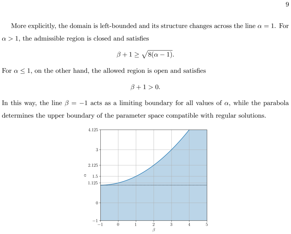
Recognition: unknown
Generalized BPS magnetic monopoles in inhomogeneous Yang-Mills-Higgs models
Pith reviewed 2026-05-09 23:59 UTC · model grok-4.3
The pith
Generalized Yang-Mills-Higgs models admit regular BPS monopoles for power-law inhomogeneities in a determined region of parameter space.
A machine-rendered reading of the paper's core claim, the machinery that carries it, and where it could break.
Core claim
By imposing the product of the generalized permittivity and permeability to equal unity, the model retains a BPS bound. For permeabilities of the form f(r)/H^α with f(r) = r^β, regular BPS monopoles exist in a specific domain of the (α, β) plane, with exact closed-form solutions available when α equals 1.
What carries the argument
The constraint that the product of the generalized permittivity P and permeability M equals one, which keeps the energy bounded below by the topological charge and reduces the equations to first order.
If this is right
- Regular monopole solutions exist for a range of exponents α and β in the power-law profile.
- Along the line α=1 the equations integrate exactly, giving closed-form expressions for the monopole fields in the inhomogeneous background.
- The energy density can exhibit single peaks, multiple concentric peaks, or be concentrated near the origin or in shells.
- Numerical solutions fill in the parameter space away from the integrable line.
Where Pith is reading between the lines
- This approach could be used to model monopoles in materials with radially varying properties, such as graded dielectrics or superconductors.
- Multi-shell configurations might correspond to bound states or resonances in the inhomogeneous medium.
- The exact solutions for α=1 provide a benchmark for testing numerical methods in more general inhomogeneous settings.
Load-bearing premise
The model requires the product of the generalized permittivity and permeability to be tuned to exactly one so that the BPS bound remains saturated.
What would settle it
Failure to find regular solutions numerically in the claimed domain of the (α, β) plane, or explicit substitution showing that the closed-form expressions for α=1 do not satisfy the first-order equations.
Figures


read the original abstract
We present a non-Abelian model for magnetic monopoles in inhomogeneous media, based on a generalization of the standard 't~Hooft-Polyakov model. The medium is described by spatially dependent couplings in the gauge and scalar sectors, constrained by $P(|\Phi|,r)M(|\Phi|,r)=1$ so that the Bogomol'nyi-Prasad-Sommerfield (BPS) bound is preserved. For static spherically symmetric configurations, we study the first-order monopole equations for the class of generalized permeabilities $M(H,r)=f(r)/H^\alpha$. For the power-law profile $f(r)=r^\beta$, we determine the domain in the $(\alpha,\beta)$ plane where regular BPS solutions exist. On the line $\alpha=1$, the system becomes exactly integrable, with closed-form monopole solutions in an inhomogeneous background. Away from this analytical sector, the solutions are constructed numerically. The model supports a rich spectrum of configurations, including effectively point-like monopoles, compact-core monopoles, hollow monopoles, shell-like structures, and multi-shell monopoles characterized by multiple concentric peaks in the energy density.
Editorial analysis
A structured set of objections, weighed in public.
Referee Report
Summary. The manuscript presents a generalization of the 't Hooft-Polyakov monopole model to inhomogeneous media by introducing spatially dependent couplings in the Yang-Mills and Higgs sectors, subject to the constraint P(|Φ|, r) M(|Φ|, r) = 1 that preserves the BPS bound. For static spherically symmetric configurations, the authors derive the first-order BPS equations for the class of permeabilities M(H, r) = f(r)/H^α with power-law f(r) = r^β. They identify the region in the (α, β) parameter plane where regular solutions exist, provide exact analytic solutions when α = 1, and construct numerical solutions otherwise. The resulting configurations include point-like, compact, hollow, shell-like, and multi-shell monopoles.
Significance. If the results hold, the work provides a controlled extension of BPS monopoles to inhomogeneous backgrounds while retaining first-order equations and the energy bound. The exact integrability along α=1 yields closed-form solutions that serve as benchmarks, and the numerical survey maps a concrete domain in parameter space supporting a spectrum of distinct profiles. This construction is valuable for exploring topological defects in media with spatial variation and supplies explicit examples that can be used for further analytic or phenomenological study.
minor comments (2)
- The abstract refers to 'effectively point-like monopoles' and 'hollow monopoles'; a short parenthetical definition in terms of the radial energy-density profile (e.g., location of the peak relative to the core radius) would improve immediate readability.
- [§4] In the numerical section, the boundary conditions imposed at r=0 and r→∞ to enforce regularity and finite energy should be stated explicitly, together with the integrator and tolerance used to delineate the (α,β) domain.
Simulated Author's Rebuttal
We thank the referee for their positive and accurate summary of our manuscript, as well as for recommending acceptance. Their assessment correctly identifies the key features of the generalized BPS monopoles in inhomogeneous Yang-Mills-Higgs models.
Circularity Check
No significant circularity; derivation self-contained
full rationale
The paper defines its model by explicitly imposing the algebraic constraint P(|Φ|,r)M(|Φ|,r)=1 as part of the construction to enforce preservation of the BPS bound and reduce to first-order equations. It then substitutes the specific ansatz M(H,r)=f(r)/H^α with power-law f(r)=r^β, integrates the resulting ODEs (analytically on α=1, numerically elsewhere), and reports the domain of regular solutions together with the observed profile types. No output quantity is used to define or fit an input parameter, no self-citation supplies a load-bearing uniqueness theorem, and the claimed spectrum follows directly from solving the stated equations rather than from any renaming or re-derivation of the inputs themselves.
Axiom & Free-Parameter Ledger
free parameters (2)
- α
- β
axioms (2)
- domain assumption P(|Φ|,r) M(|Φ|,r)=1 preserves the BPS bound
- domain assumption Static spherically symmetric field configurations
Reference graph
Works this paper leans on
-
[1]
Since eH(0) = 0 and eK(0) = 1, we may write eH(ξ) =δ eH(ξ), eK(ξ) = 1−δ eK(ξ)
Nearξ= 0 Near the origin, it is convenient to introduce the deviations δ eH(ξ)≡ eH(0)− eH(ξ) , δ eK(ξ)≡ eK(0)− eK(ξ) ,(A5) which vanish atξ= 0 and grow toward unity asξ→1, consistent with (A4). Since eH(0) = 0 and eK(0) = 1, we may write eH(ξ) =δ eH(ξ), eK(ξ) = 1−δ eK(ξ). For regular monopole solutions, both eH(ξ) and eK(ξ) must approach their boundary va...
-
[2]
∞X k=0 β k (−t)k # ∞X n=0 ( ¯H1−α)(n)(0) n! tn ! dt = ∞Y k,n=0 exp ( β k (−1)k ( ¯H1−α)(n)(0) n!
Nearξ= 1 To analyze the behavior of the solutions near spatial infinity, we introduce the variable τ≡1−ξ,(A12) so thatτ→0 corresponds tor→ ∞. We further define ¯H(τ)≡ eH(ξ(τ)), ¯K(τ)≡ eK(ξ(τ)).(A13) 25 In terms of these variables, the BPS equations can be written as ¯K(τ) = exp Z τ 1 t−(β+2)(1−t) β ¯H 1−α(t) dt ,(A14a) ¯K2 = 1 +τ −β(1−τ) β+2 ¯H −α ¯H ′,(A...
-
[3]
(A11), up tor=r b
One way to proceed is defining this parameter as the root of a function shooting(a0), constructed as follows: for a given trial value ofa 0, the BPS system is integrated from the initial conditions (H a, Ka) atr=r a, specified by Eq. (A11), up tor=r b. The function shooting(a0) then returns the mismatch shooting(a0) =H tar −H b,(A24) whereH b denotes the ...
-
[4]
Armend´ ariz-Pic´ on, T
C. Armend´ ariz-Pic´ on, T. Damour, and V. Mukhanov, Physics Letters B458, 209 (1999), ISSN 0370- 2693, URLhttps://www.sciencedirect.com/science/article/pii/S0370269399006036
1999
-
[5]
E. Babichev, Phys. Rev. D74, 085004 (2006), URLhttps://link.aps.org/doi/10.1103/PhysRevD. 74.085004
-
[6]
C. Adam, J. S´ anchez-Guill´ en, and A. Wereszczy´ nski, Journal of Physics A: Mathematical and Theo- retical40, 13625 (2007), URLhttps://doi.org/10.1088/1751-8113/40/45/009
-
[7]
C. Adam, J. Sanchez-Guillen, and A. Wereszczynski, Journal of Physics A: Mathematical and Theo- retical42, 089801 (2009), URLhttps://doi.org/10.1088/1751-8121/42/8/089801
-
[8]
Manifestly crossing-invariant parametrization of n-meson amplitude,
G. ’t Hooft, Nuclear Physics B79, 276 (1974), ISSN 0550-3213, URLhttps://www.sciencedirect. com/science/article/pii/0550321374904866
-
[9]
A. M. Polyakov, JETP Lett.20, 194 (1974), [Pisma Zh. Eksp. Teor. Fiz. 20, 430 (1974)]
1974
-
[10]
E. B. Bogomolny, Sov. J. Nucl. Phys.24, 449 (1976), [Yad. Fiz. 24, 861 (1976)]
1976
-
[11]
M. K. Prasad and C. M. Sommerfield, Phys. Rev. Lett.35, 760 (1975), URLhttps://link.aps.org/ doi/10.1103/PhysRevLett.35.760
-
[12]
R. Casana, M. M. Ferreira, and E. da Hora, Phys. Rev. D86, 085034 (2012), URLhttps://link. aps.org/doi/10.1103/PhysRevD.86.085034
-
[13]
A. N. Atmaja and I. Prasetyo, Advances in High Energy Physics2018, 7376534 (2018), URLhttps: //doi.org/10.1155/2018/7376534
-
[14]
A. N. Atmaja, Eur. Phys. J. C82, 602 (2022), URLhttps://doi.org/10.1140/epjc/ s10052-022-10569-6
-
[15]
Mulyanto, E. S. Fadhilla, and A. N. Atmaja, Physics Letters B874, 140267 (2026), ISSN 0370-2693, URLhttps://doi.org/10.1016/j.physletb.2026.140267
-
[16]
Bazeia, R
D. Bazeia, R. Casana, M. Ferreira, E. da Hora, and L. Losano, Physics Letters B727, 548 (2013), ISSN 0370-2693, URLhttps://www.sciencedirect.com/science/article/pii/S0370269313008939
2013
-
[17]
D. Bazeia, M. A. Marques, and R. Menezes, Phys. Rev. D97, 105024 (2018), URLhttps://link. aps.org/doi/10.1103/PhysRevD.97.105024
-
[18]
D. Bazeia, M. A. Marques, and G. J. Olmo, Phys. Rev. D98, 025017 (2018), URLhttps://link. aps.org/doi/10.1103/PhysRevD.98.025017
-
[19]
D. Bazeia, M. A. Marques, and R. Menezes, Phys. Rev. D98, 065003 (2018), URLhttps://link. aps.org/doi/10.1103/PhysRevD.98.065003
-
[20]
D. Bazeia, M. A. Liao, and M. A. Marques, The European Physical Journal C81, 552 (2021), URL https://doi.org/10.1140/epjc/s10052-021-09352-w
-
[21]
Beneˇ s and F
P. Beneˇ s and F. Blaschke, Phys. Rev. D107, 125002 (2023), URLhttps://link.aps.org/doi/10. 1103/PhysRevD.107.125002
2023
-
[22]
P. Beneˇ s and F. Blaschke, Progress of Theoretical and Experimental Physics2026, 023B04 (2026), 30 ISSN 2050-3911, URLhttps://doi.org/10.1093/ptep/ptag004
-
[23]
C. Adam, J. M. Queiruga, and A. Wereszczynski, J. High Energ. Phys.07, 164 (2019), URLhttps: //doi.org/10.1007/JHEP07(2019)164
-
[24]
C. Adam, T. Romanczukiewicz, and A. Wereszczynski, J. High Energ. Phys.03, 131 (2019), URL https://doi.org/10.1007/JHEP03(2019)131
-
[25]
C. Adam, K. Oles, J. M. Queiruga, T. Romanczukiewicz, and A. Wereszczynski, J. High Energ. Phys. 07, 150 (2019), URLhttps://doi.org/10.1007/JHEP07(2019)150
-
[26]
J. a. G. F. Campos and A. Mohammadi, Phys. Rev. D102, 045003 (2020), URLhttps://link.aps. org/doi/10.1103/PhysRevD.102.045003
-
[27]
S lawi´ nska, Phys
K. S lawi´ nska, Phys. Rev. E111, 014228 (2025), URLhttps://link.aps.org/doi/10.1103/ PhysRevE.111.014228
2025
-
[28]
Tong and K
D. Tong and K. Wong, J. High Energ. Phys.01, 090 (2014), URLhttps://doi.org/10.1007/ JHEP01(2014)090
2014
-
[29]
A. Cockburn, S. Krusch, and A. A. Muhamed, J. Math. Phys.58, 063509 (2017), URLhttps://doi. org/10.1063/1.4984980
-
[30]
V. Almeida, R. Casana, E. da Hora, and S. Krusch, Phys. Rev. D106, 016010 (2022), URLhttps: //link.aps.org/doi/10.1103/PhysRevD.106.016010
-
[31]
D. Bazeia, J. G. F. Campos, and A. Mohammadi, J. High Energ. Phys.12, 108 (2024), URLhttps: //doi.org/10.1007/JHEP12(2024)108
-
[32]
N. H. Gonzalez-Gutierrez, R. Casana, and A. C. Santos, J. High Energ. Phys.01, 005 (2026), URL https://doi.org/10.1007/JHEP01(2026)005
-
[33]
D. Bazeia, M. A. Marques, and R. Menezes, Eur. Phys. J. C85, 836 (2025), URLhttps://doi.org/ 10.1140/epjc/s10052-025-14582-3
- [34]
discussion (0)
Sign in with ORCID, Apple, or X to comment. Anyone can read and Pith papers without signing in.