Recognition: unknown
A Hough transform approach to safety-aware scalar field mapping using Gaussian Processes
Pith reviewed 2026-05-10 00:05 UTC · model grok-4.3
The pith
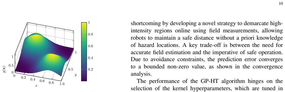
A robot maps unknown scalar fields safely by combining Gaussian process models with real-time Hough transform estimates of high-intensity danger zones.
A machine-rendered reading of the paper's core claim, the machinery that carries it, and where it could break.
Core claim
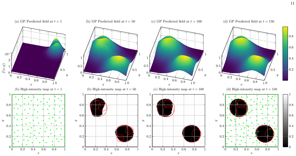
By running the Hough transform on the current Gaussian process posterior, the spatial geometry of high-intensity unsafe regions can be recovered in real time; this geometry supplies both a safe-sampling criterion that keeps the robot away from danger zones with high probability and a set of constraints for subsequent motion planning.
What carries the argument
The Hough transform applied to the evolving GP posterior, which converts the probabilistic field estimate into explicit geometric descriptions of unsafe regions.
If this is right
- The robot can continue collecting measurements while maintaining a user-specified probability of never entering an unsafe region.
- Motion planners can treat the Hough-extracted boundaries as hard obstacles whose locations improve as more data arrive.
- The same posterior-plus-Hough pipeline supplies both mapping accuracy and safety certificates without requiring a separate safety layer.
- Numerical simulations and the indoor light-mapping experiment show that the combined method produces usable maps and feasible paths.
Where Pith is reading between the lines
- The method could be extended to time-varying fields if the GP is replaced by a spatio-temporal kernel while the Hough step remains unchanged.
- The same safety-aware loop might apply to other sensors whose output can be modeled by a GP, such as temperature or radiation mapping.
- Because the Hough transform operates on the posterior mean or thresholded probability map, any GP approximation that preserves closed-form predictive statistics could be substituted without redesigning the safety logic.
Load-bearing premise
The spatial structure of high-intensity regions can be recovered reliably and quickly enough by applying the Hough transform to the current Gaussian process posterior.
What would settle it
Run the same robot and sensor in a known environment containing a single compact high-intensity patch and check whether the Hough-extracted boundary matches the true patch boundary within the uncertainty reported by the GP at each time step.
Figures


read the original abstract
This paper presents a framework for mapping unknown scalar fields using a sensor-equipped autonomous robot operating in unsafe environments. The unsafe regions are defined as regions of high-intensity, where the field value exceeds a predefined safety threshold. For safe and efficient mapping of the scalar field, the sensor-equipped robot must avoid high-intensity regions during the measurement process. In this paper, the scalar field is modeled as a sample from a Gaussian process (GP), which enables Bayesian inference and provides closed-form expressions for both the predictive mean and the uncertainty. Concurrently, the spatial structure of the high-intensity regions is estimated in real-time using the Hough transform (HT), leveraging the evolving GP posterior. A safe sampling strategy is then employed to guide the robot towards safe measurement locations, using probabilistic safety guarantees on the evolving GP posterior. The estimated high-intensity regions also facilitate the design of safe motion plans for the robot. The effectiveness of the approach is verified through two numerical simulation studies and an indoor experiment for mapping a light-intensity field using a wheeled mobile robot.
Editorial analysis
A structured set of objections, weighed in public.
Referee Report
Summary. The paper presents a framework for mapping unknown scalar fields using a sensor-equipped autonomous robot in unsafe environments, where unsafe regions are defined as high-intensity areas exceeding a safety threshold. The scalar field is modeled as a Gaussian process (GP) to enable Bayesian inference with closed-form predictive mean and variance. The Hough transform is applied in real-time to the evolving GP posterior to estimate the spatial structure of high-intensity regions. This estimate supports a safe sampling strategy that guides the robot to safe measurement locations using probabilistic safety guarantees, and also aids in designing safe motion plans. Effectiveness is demonstrated via two numerical simulation studies and an indoor experiment mapping a light-intensity field with a wheeled mobile robot.
Significance. If the Hough transform step can be shown to preserve the GP's probabilistic bounds, the approach would offer a practical way to combine Bayesian field estimation with geometric feature detection for real-time safe exploration in hazardous environments. The inclusion of both simulations and a physical experiment provides empirical grounding, and the use of standard GP inference plus a classical transform like HT makes the method potentially accessible for robotics applications.
major comments (3)
- [Framework description (Hough transform application to GP posterior)] The central construction that converts the GP posterior (mean and variance) into an input for the Hough transform (via thresholding or level-set extraction) is load-bearing for the safety claims, yet no derivation is provided showing that the resulting region estimate preserves the required probabilistic bounds such as P(field > threshold) < ε along planned paths or sampling locations.
- [Safe sampling strategy and motion planning] The safe sampling strategy and motion planning sections rely on the HT-detected high-intensity regions to enforce probabilistic safety, but the manuscript does not address how discretization or the parametric assumption (lines/circles) affects tail probability mass when the true unsafe regions are non-parametric or irregular.
- [Numerical simulations and indoor experiment] The verification via simulations and experiment reports effectiveness but provides no quantitative comparison to a baseline GP-only approach (without HT) or detailed error analysis on how often the safety threshold is violated, weakening the support for the claim that the combined method delivers reliable probabilistic guarantees.
minor comments (2)
- [Abstract] The abstract states that 'probabilistic safety guarantees' are used but does not define the precise form of the guarantee (e.g., the numerical value of the risk threshold ε or the exact probability statement).
- [Methods] Notation for the GP posterior discretization step prior to HT input should be clarified, including how variance is incorporated into the binary or weighted image.
Simulated Author's Rebuttal
We thank the referee for the thoughtful and constructive review of our manuscript. The comments highlight important aspects of the probabilistic guarantees and empirical validation that we will address in the revision. We provide point-by-point responses below.
read point-by-point responses
-
Referee: [Framework description (Hough transform application to GP posterior)] The central construction that converts the GP posterior (mean and variance) into an input for the Hough transform (via thresholding or level-set extraction) is load-bearing for the safety claims, yet no derivation is provided showing that the resulting region estimate preserves the required probabilistic bounds such as P(field > threshold) < ε along planned paths or sampling locations.
Authors: We agree that the manuscript lacks a formal derivation demonstrating that the Hough transform step preserves the GP's probabilistic bounds. The current approach thresholds the predictive mean to generate an input image for the Hough transform and uses the detected parametric features to delineate avoidance zones. This step is heuristic rather than a direct probabilistic mapping. In the revised manuscript we will add a dedicated subsection discussing the approximation, its potential impact on tail probabilities, and the conservative safety margins that result in practice. We will also include a brief analysis showing that the method tends to over-estimate unsafe regions in the tested scenarios. revision: partial
-
Referee: [Safe sampling strategy and motion planning] The safe sampling strategy and motion planning sections rely on the HT-detected high-intensity regions to enforce probabilistic safety, but the manuscript does not address how discretization or the parametric assumption (lines/circles) affects tail probability mass when the true unsafe regions are non-parametric or irregular.
Authors: The referee correctly notes that the parametric (line/circle) assumption and discretization inherent to the Hough transform can distort the representation of irregular unsafe regions and thereby influence the effective tail probabilities used for safety. We will revise the safe sampling and motion planning sections to explicitly acknowledge these limitations, provide a qualitative discussion of how discretization grid resolution affects detected boundaries, and note that the approach is most appropriate when unsafe regions admit approximate parametric descriptions. Sensitivity analysis with respect to discretization parameters will be added to the supplementary material. revision: partial
-
Referee: [Numerical simulations and indoor experiment] The verification via simulations and experiment reports effectiveness but provides no quantitative comparison to a baseline GP-only approach (without HT) or detailed error analysis on how often the safety threshold is violated, weakening the support for the claim that the combined method delivers reliable probabilistic guarantees.
Authors: We accept that the evaluation would be strengthened by direct quantitative comparisons and explicit violation statistics. In the revised manuscript we will augment both simulation studies with a GP-only baseline (using the same predictive mean and variance but without Hough-transform-based region detection). We will report additional metrics including the number and magnitude of threshold violations, the fraction of safe samples obtained, and mapping coverage efficiency. For the indoor experiment we will include a post-hoc analysis of the measured light-intensity values relative to the safety threshold along the executed trajectory. revision: yes
Circularity Check
No significant circularity; modular GP posterior + HT pipeline
full rationale
The paper models the scalar field via standard GP regression, yielding closed-form posterior mean and variance. It then applies the Hough transform to the evolving posterior (via thresholding or level-set extraction) to estimate high-intensity region geometry, and feeds the resulting estimates into a separate safe sampling planner that enforces probabilistic bounds P(field > threshold) < ε. No equation reduces a prediction to a fitted parameter by construction, no self-citation supplies a uniqueness theorem or ansatz, and the safety guarantees remain independent of the HT step. The derivation chain is therefore self-contained and externally falsifiable.
Axiom & Free-Parameter Ledger
free parameters (1)
- safety threshold
axioms (2)
- domain assumption Scalar field can be modeled as a sample from a Gaussian process
- domain assumption High-intensity regions possess spatial structure detectable by Hough transform
Reference graph
Works this paper leans on
-
[1]
A rendering algorithm for visualizing 3D scalar fields,
P. Sabella, “A rendering algorithm for visualizing 3D scalar fields,” Comp. Graph., p. 51–58, Jun. 1988
1988
-
[2]
Kalman filter based large-scale wildfire monitoring with a system of UA Vs,
Z. Lin, H. H. T. Liu, and M. Wotton, “Kalman filter based large-scale wildfire monitoring with a system of UA Vs,”IEEE Trans. Ind. Electron., vol. 66, no. 1, pp. 606–615, Jan. 2019
2019
-
[3]
New assessment method for solar radiation effects on indoor thermal comfort based on scalar irradiance - using volume photon mapping,
K. Matsuda, K. Nozaki, R. Schregle, K. Takase, K. Taniguchi, and N. Yoshizawa, “New assessment method for solar radiation effects on indoor thermal comfort based on scalar irradiance - using volume photon mapping,”Build. Environ., vol. 243, p. 110662, 2023
2023
-
[4]
Efficient two-dimensional scalar fields reconstruction of laminar flames from infrared hyperspectral measurements with a machine learning approach,
T. Ren, H. Li, M. F. Modest, and C. Zhao, “Efficient two-dimensional scalar fields reconstruction of laminar flames from infrared hyperspectral measurements with a machine learning approach,”J. Quant. Spectrosc. Radiat. Transfer, vol. 271, p. 107724, 2021
2021
-
[5]
Estimating scalar fields with mobile sensor networks,
R. A. Razak, S. Sukumar, and H. Chung, “Estimating scalar fields with mobile sensor networks,” inProc. Ind. Control Conf., 2019, pp. 63–68
2019
-
[6]
Cooperative and active sensing in mobile sensor networks for scalar field mapping,
H. M. La, W. Sheng, and J. Chen, “Cooperative and active sensing in mobile sensor networks for scalar field mapping,”IEEE Trans. Syst., Man, Cybern., Syst., vol. 45, no. 1, pp. 1–12, 2015
2015
-
[7]
A high-speed, light-weight scalar magnetometer bird for km scale UA V magnetic surveying: on sensor choice, bird design, and quality of output data,
A. Dossing, E. L. S. Silva, G. Martelet, and Rasmussen, “A high-speed, light-weight scalar magnetometer bird for km scale UA V magnetic surveying: on sensor choice, bird design, and quality of output data,” Remote Sensing, vol. 4, no. 4, 2021
2021
-
[8]
Distributed sensor fusion for scalar field mapping using mobile sensor networks,
H. M. La and W. Sheng, “Distributed sensor fusion for scalar field mapping using mobile sensor networks,”IEEE Trans. Cybern., vol. 43, no. 2, pp. 766–778, Apr. 2013
2013
-
[9]
A distributed scalar field mapping strategy for mobile robots,
T. X. Lin, S. Al-Abri, S. Coogan, and F. Zhang, “A distributed scalar field mapping strategy for mobile robots,” inProc. Int. Conf. Intell. Robots Syst., 2020, pp. 11 581–11 586
2020
-
[10]
Compressive and collab- orative mobile sensing for scalar field mapping in robotic networks,
M. T. Nguyen, H. M. La, and K. A. Teague, “Compressive and collab- orative mobile sensing for scalar field mapping in robotic networks,” in Proc. Annu. Allerton Conf. Commun., Control, Comput.IEEE, Sep. 2015, pp. 873–880
2015
-
[11]
Robotic exploration of an unknown nuclear environment using radiation informed autonomous navigation,
K. Groves, E. Hernandez, A. West, T. Wright, and B. Lennox, “Robotic exploration of an unknown nuclear environment using radiation informed autonomous navigation,”Robotics, vol. 10, no. 2, p. 78, May 2021
2021
-
[12]
Detection of nuclear sources by UA V teleoperation using a visuo-haptic augmented reality interface,
J. Aleotti, G. Micconi, S. Caselli, G. Benassi, N. Zambelli, M. Bettelli, and A. Zappettini, “Detection of nuclear sources by UA V teleoperation using a visuo-haptic augmented reality interface,”Sensors, vol. 17, no. 10, p. 2234, Sep. 2017
2017
-
[13]
Cooperative control of multiple UA Vs for forest fire monitoring and detection,
K. A. Ghamry and Y . Zhang, “Cooperative control of multiple UA Vs for forest fire monitoring and detection,” inProc. Int. Conf. Mechatronic Embedded Syst. Appl.IEEE, Aug. 2016. 11 0 0.2 0.4 0.6 0.8 1 0 0.5 1 0 1 2 ·10−2 x y f (x, y) (a) GP Predicted field at t = 1 0 0.2 0.4 0.6 0.8 1 0 0.5 1 0 0.5 1 x y (b) GP Predicted field at t = 50 0 0.2 0.4 0.6 0.8 ...
2016
-
[14]
Forest fire monitoring with multiple small uavs,
D. Casbeer, S.-M. Li, R. Beard, R. Mehra, and T. McLain, “Forest fire monitoring with multiple small uavs,” inProc. Am. Cont. Conf.IEEE, 2015, pp. 3530–3535
2015
-
[15]
Distributed estimation of fields using a sensor network with quantized measurements,
C. Jayasekaramudeli, A. S. Leong, A. T. Skvortsov, D. J. Nielsen, and O. Ilaya, “Distributed estimation of fields using a sensor network with quantized measurements,”Sensors, vol. 24, no. 16, 2024
2024
-
[16]
Stability of extremum seeking feedback for general nonlinear dynamic systems,
M. Krsti ´c and H.-H. Wang, “Stability of extremum seeking feedback for general nonlinear dynamic systems,”Automatica, vol. 36, no. 4, pp. 595–601, Apr. 2000
2000
-
[17]
K. B. Ariyur and M. Krsti ´c,Real-Time Optimization by Extremum- Seeking Control. Wiley, Sep. 2003
2003
-
[18]
Multivariable Newton-based extremum seeking,
A. Ghaffari, M. Krsti ´c, and D. Ne ˇsi´c, “Multivariable Newton-based extremum seeking,”Automatica, vol. 48, no. 8, pp. 1759–1767, Aug. 2012
2012
-
[19]
Practically safe extremum seeking,
A. Williams, M. Krsti ´c, and A. Scheinker, “Practically safe extremum seeking,” inProc. IEEE Conf. Decis. Control, 2022, pp. 1993–1998. 12 0 2 4 6 8 10 0 2 4 6 8 10 0 5 10 x y z Fig. 7: The estimated high-intensity regions in the domain. The planned measurement locations detected in estimated high- intensity regions are also shown as black dots. Fig. 8: ...
2022
-
[20]
Semiglobal safety-filtered extremum seeking with unknown CBFs,
——, “Semiglobal safety-filtered extremum seeking with unknown CBFs,”IEEE Trans. Autom. Control, vol. 70, no. 3, pp. 1698–1713, 2025
2025
-
[21]
Obstacle avoidance and path planning methods for autonomous navigation of mobile robot,
K. Katona, H. A. Neamah, and P. Korondi, “Obstacle avoidance and path planning methods for autonomous navigation of mobile robot,”Sensors, vol. 24, no. 11, p. 3573, Jun. 2024
2024
-
[22]
Path planning and obstacle avoidance for autonomous mobile robots: A review,
V . Kunchev, L. Jain, V . Ivancevic, and A. Finn, “Path planning and obstacle avoidance for autonomous mobile robots: A review,” inProc. Knowl.-Based Intell. Inf. & Eng. Syst., B. Gabrys, R. J. Howlett, and L. C. Jain, Eds. Berlin, Heidelberg: Springer Berlin Heidelberg, 2006, pp. 537–544
2006
-
[23]
Minguez, F
J. Minguez, F. Lamiraux, and J.-P. Laumond,Motion Planning and Obstacle Avoidance. Berlin, Heidelberg: Springer Berlin Heidelberg, 2008, pp. 827–852
2008
-
[24]
Self- configuring robot path planning with obstacle avoidance via deep reinforcement learning,
B. Sangiovanni, G. P. Incremona, M. Piastra, and A. Ferrara, “Self- configuring robot path planning with obstacle avoidance via deep reinforcement learning,”IEEE Control Syst. Lett., vol. 5, no. 2, pp. 397– 402, 2021
2021
-
[25]
Multi-robot source location of scalar fields by a novel swarm search mechanism with collision/obstacle avoidance,
R.-G. Li and H.-N. Wu, “Multi-robot source location of scalar fields by a novel swarm search mechanism with collision/obstacle avoidance,” IEEE Trans. Intell. Transp. Syst., vol. 23, no. 1, pp. 249–264, Jan. 2022
2022
-
[26]
Safety-critical planning and control for dynamic obstacle avoidance using control barrier functions,
S. Liu, Y . Mao, and C. A. Belta, “Safety-critical planning and control for dynamic obstacle avoidance using control barrier functions,” in2025 American Control Conference (ACC), 2025, pp. 348–354
2025
-
[27]
C. E. Rasmussen and C. K. I. Williams,Gaussian processes for machine learning.Cambridge, MA: MIT Press, 2006
2006
-
[28]
Informative path planning for an autonomous underwater vehicle,
J. Binney, A. Krause, and G. S. Sukhatme, “Informative path planning for an autonomous underwater vehicle,” inProc. IEEE Int. Conf. Robot. Autom., May 2010, pp. 4791–4796
2010
-
[29]
Adaptive continuous-space informative path planning for online envi- ronmental monitoring,
G. Hitz, E. Galceran, M.- `E. Garneau, F. Pomerleau, and R. Siegwart, “Adaptive continuous-space informative path planning for online envi- ronmental monitoring,”J. Field Robot., vol. 34, no. 8, pp. 1427–1449, May 2017
2017
-
[30]
Comparative study of Hough transform methods for circle finding,
H. Yuen, J. Princen, J. Illingworth, and J. Kittler, “Comparative study of Hough transform methods for circle finding,”Image Vision Comput., vol. 8, no. 1, pp. 71–77, Feb. 1990
1990
-
[31]
Use of the Hough transformation to detect lines and curves in pictures,
R. O. Duda and P. E. Hart, “Use of the Hough transformation to detect lines and curves in pictures,”Commun., vol. 15, no. 1, pp. 11–15, Jan. 1972
1972
-
[32]
Scalar field mapping with adaptive high-intensity region avoidance,
M. Qureshi, T. E. Ogri, Z. I. Bell, and R. Kamalapurkar, “Scalar field mapping with adaptive high-intensity region avoidance,” inProc. IEEE Conf. Control Technol. Appl.IEEE, Aug. 2024, pp. 388–393
2024
-
[33]
Bayesian experimental design: A review,
K. Chaloner and I. Verdinelli, “Bayesian experimental design: A review,” Statist. Sci., vol. 10, no. 3, Aug. 1995
1995
-
[34]
Sampling-based algorithms for optimal motion planning,
S. Karaman and E. Frazzoli, “Sampling-based algorithms for optimal motion planning,”Int. J. Robot. Res., vol. 30, no. 7, pp. 846–894, Jun. 2011
2011
-
[35]
Sch ¨olkopf and A
B. Sch ¨olkopf and A. J. Smola,Learning with Kernels: Support Vector Machines, Regularization, Optimization, and Beyond. The MIT Press, Dec. 2001
2001
-
[36]
Information- theoretic regret bounds for Gaussian process optimization in the bandit setting,
N. Srinivas, A. Krause, S. M. Kakade, and M. W. Seeger, “Information- theoretic regret bounds for Gaussian process optimization in the bandit setting,”IEEE Trans. Inf. Theory, pp. 3250–3265, May 2012
2012
-
[37]
Kalman filter-based large-scale wildfire monitoring with a system of UA Vs,
Z. Lin, H. H. T. Liu, and M. Wotton, “Kalman filter-based large-scale wildfire monitoring with a system of UA Vs,”IEEE Trans Ind Electron, vol. 66, no. 1, pp. 606–615, Jan. 2019
2019
-
[38]
A survey on forest fire monitoring using unmanned aerial vehicles,
F. A. Hossain, Y . Zhang, and C. Yuan, “A survey on forest fire monitoring using unmanned aerial vehicles,” inProc. Int. Symp. Autom. Syst. (ISAS), 2019, pp. 484–489
2019
-
[39]
Cooperative control of UA Vs for localization of intermittently emitting mobile targets,
D. J. Pack, P. DeLima, G. J. Toussaint, and G. York, “Cooperative control of UA Vs for localization of intermittently emitting mobile targets,”Trans. Sys. Man Cyber., vol. 39, no. 4, p. 959–970, Aug. 2009
2009
-
[40]
Autonomous search of radioactive sources through mobile robots,
J. Huo, M. Liu, K. A. Neusypin, H. Liu, M. Guo, and Y . Xiao, “Autonomous search of radioactive sources through mobile robots,” Sensors, vol. 20, no. 12, 2020
2020
-
[41]
Autonomous exploration for radioactive hotspots localization taking account of sensor limitations,
H. Ardiny, S. Witwicki, and F. Mondada, “Autonomous exploration for radioactive hotspots localization taking account of sensor limitations,” Sensors, vol. 19, no. 2, 2019
2019
-
[42]
Small teleoperated robot for nuclear radiation and chemical leak detection,
K. Qian, A. Song, J. Bao, and H. Zhang, “Small teleoperated robot for nuclear radiation and chemical leak detection,”Int. J. Adv. Robot. Syst., vol. 9, no. 3, p. 70, 2012
2012
-
[43]
T. M. Cover and J. A. Thomas,Information Theory and Statistics. John Wiley & Sons, Ltd, Oct. 2005, ch. 11, pp. 347–408
2005
-
[44]
An exact algorithm for maximum entropy sampling,
C.-W. Ko, J. Lee, and M. Queyranne, “An exact algorithm for maximum entropy sampling,”Oper. Res., no. 4, pp. 684–691, Aug. 1995. 13 -4 -2 0 2 4 6 x (m) -2 -1.5 -1 -0.5 0 0.5 1 1.5y (m) 40 60 80 100 120 140 160 (a) Initial position: bottom-left -4 -2 0 2 4 6 x (m) -2 -1.5 -1 -0.5 0 0.5 1 1.5y (m) 20 40 60 80 100 120 140 160 (b) Initial position: bottom-rig...
1995
-
[45]
Near-optimal nonmyopic value of information in graphical models.arXiv preprint arXiv:1207.1394, 2012
A. Krause and C. E. Guestrin, “Near-optimal nonmyopic value of infor- mation in graphical models,” 2012, arXiv preprint, arXiv:1207.1394
-
[46]
An analysis of approximations for maximizing submodular set functions–I,
G. L. Nemhauser, L. A. Wolsey, and M. L. Fisher, “An analysis of approximations for maximizing submodular set functions–I,”Math. Program., no. 1, pp. 265–294, 1978
1978
-
[47]
Near-optimal sensor placements in Gaussian processes: Theory, efficient algorithms and empirical stud- ies,
A. Krause, A. Singh, and C. Guestrin, “Near-optimal sensor placements in Gaussian processes: Theory, efficient algorithms and empirical stud- ies,”J. Mach. Learn. Res., vol. 9, no. 8, pp. 235–284, 2008
2008
-
[48]
D. L. Applegate, R. E. Bixby, V . Chvat ´al, and W. J. Cook,The Traveling Salesman Problem: A Computational Study. Princeton University Press, 2006
2006
-
[49]
Nearest neighbor pattern classification,
T. Cover and P. Hart, “Nearest neighbor pattern classification,”IEEE Trans. Inf. Theory, vol. 13, no. 1, pp. 21–27, 1967
1967
-
[50]
Wendland,Scattered data approximation
H. Wendland,Scattered data approximation. Cambridge University Press, 2004
2004
-
[51]
Chomp: Gradient optimization techniques for efficient motion planning,
N. Ratliff, M. Zucker, J. A. Bagnell, and S. Srinivasa, “Chomp: Gradient optimization techniques for efficient motion planning,” inProc. IEEE Int. Conf. Robot. Autom., 2009, pp. 489–494
2009
-
[52]
Stomp: Stochastic trajectory optimization for motion planning,
M. Kalakrishnan, S. Chitta, E. Theodorou, P. Pastor, and S. Schaal, “Stomp: Stochastic trajectory optimization for motion planning,” in Proc. IEEE Int. Conf. Robot. Autom., 2011, pp. 4569–4574
2011
-
[53]
Finding locally optimal, collision-free trajectories with sequential convex optimization,
J. Schulman, J. Ho, A. X. Lee, I. Awwal, H. Bradlow, and P. Abbeel, “Finding locally optimal, collision-free trajectories with sequential convex optimization,”Proc. Robot.: Sci. Syst., 2013
2013
-
[54]
On the convergence of generalized kernel- based interpolation by greedy data selection algorithms,
K. Albrecht and A. Iske, “On the convergence of generalized kernel- based interpolation by greedy data selection algorithms,”BIT Numer. Math., vol. 65, 2025
2025
discussion (0)
Sign in with ORCID, Apple, or X to comment. Anyone can read and Pith papers without signing in.