Recognition: unknown
Constant Factor Analysis of Optimal Quantum Linear Solvers in Practice
Pith reviewed 2026-05-08 12:03 UTC · model grok-4.3
The pith
Numerical tests show the adiabatic quantum linear solver performs slightly better than the shortcut method when the solution norm is unknown, but the shortcut is significantly better for known-norm non-Hermitian matrices.
A machine-rendered reading of the paper's core claim, the machinery that carries it, and where it could break.
Core claim
In the numerical experiments, when the solution norm is unknown the adiabatic solver shows slightly better performance overall, while when the solution norm is known the shortcut method provides significantly better performance specifically for non-Hermitian matrices.
What carries the argument
Numerical benchmarking of the adiabatic and shortcut solvers on random matrix ensembles, which reveals the realized constant factors beyond the analytic upper bounds.
If this is right
- When the solution norm is unknown, the adiabatic solver is preferable due to its slight edge in performance.
- When the solution norm is known, the shortcut method should be used for non-Hermitian systems as it offers significantly lower constants.
- The choice between solvers can be guided by problem characteristics like matrix type and norm knowledge.
- Both methods realize much smaller constants than their analytic bounds suggest in practice.
Where Pith is reading between the lines
- If these random systems capture typical structure, then applications in quantum simulation could benefit from selecting the shortcut method when norms are available.
- Testing on matrices with specific structures from applications like finite element methods or graph Laplacians could reveal further performance differences.
- Knowing the solution norm in advance may be a key practical advantage for implementing the shortcut solver efficiently.
Load-bearing premise
The two families of random linear systems used in the tests represent the kinds of matrices that appear in real quantum computing applications.
What would settle it
Measuring the constant factors on linear systems taken from a concrete application such as quantum chemistry or machine learning and finding that the performance ordering reverses or the differences disappear.
Figures


read the original abstract
Optimal quantum linear equation solvers provide complexity $O(\kappa\log(1/\epsilon))$, where $\kappa$ is the condition number and $\epsilon$ is the allowable error. The optimal solver using a discrete adiabatic approach [PRX Quantum 3, 040303 (2022)] has large analytically proven constant factors for the upper bound on the complexity. The constant factors were later found to be about 1,200 times smaller in numerical testing [Quantum 9, 1887 (2025)]. This meant it is about an order of magnitude more efficient than using a randomised approach from [PRX Quantum 6, 040373 (2025)], which has far smaller analytically proven constant factors. Recently, a ``Shortcut'' method has been found to provide an optimal solver which also has small proven constant factors. In the present work, we conduct a comprehensive numerical analysis comparing this method with the adiabatic solver for two families of random linear systems. We find that, in the case where the solution norm is unknown, the adiabatic solver provides slightly better performance. If the solution norm is known, then the shortcut method provides significantly better performance for non-Hermitian matrices.
Editorial analysis
A structured set of objections, weighed in public.
Referee Report
Summary. The paper numerically compares the practical constant factors of two optimal quantum linear equation solvers—the discrete adiabatic method and the shortcut method—on two families of random linear systems. It reports that the adiabatic solver performs slightly better when the solution norm is unknown, while the shortcut method yields significantly better performance for non-Hermitian matrices when the solution norm is known. The work builds on prior analytic bounds and numerical findings for the adiabatic solver to offer guidance for practical use.
Significance. If the reported numerical rankings hold, the results supply concrete empirical data that can guide selection between optimal quantum linear solvers in applications, showing that numerical performance can favor the shortcut method in specific regimes even when analytic constant-factor bounds favor the adiabatic approach. This helps translate theoretical O(κ log(1/ε)) complexity into actionable implementation choices.
major comments (2)
- [Abstract and Numerical Experiments section] Abstract and Numerical Experiments section: The central claims rest on performance differences observed for 'two families of random linear systems,' yet the manuscript provides only high-level summaries of matrix generation, sparsity, eigenvalue distributions, and the precise performance metric (e.g., gate count or effective constant factor). Because analytic upper bounds are known to be loose, the practical ranking depends entirely on whether these ensembles reproduce the structural features of matrices arising in quantum applications; without those details or cross-validation against application-derived matrices (Hamiltonian simulation, discretized PDEs), the quantitative conclusions cannot be independently verified or generalized.
- [Abstract] Abstract: The distinction between 'unknown' and 'known' solution norm is central to the reported performance reversal, but the experimental protocol for controlling or estimating the norm (and any associated overhead) is not specified. This is load-bearing for the claim that the shortcut method is 'significantly better' in the known-norm non-Hermitian case, as the comparison could be sensitive to how norm knowledge is operationalized.
minor comments (1)
- [Abstract] The abstract would benefit from stating the matrix dimensions, condition-number ranges, and number of instances tested to allow readers to gauge the statistical robustness of the 'slightly' versus 'significantly' qualifiers.
Simulated Author's Rebuttal
We thank the referee for their careful reading and constructive comments on our manuscript. We address each major comment point by point below and have prepared revisions to improve the clarity and reproducibility of the work.
read point-by-point responses
-
Referee: [Abstract and Numerical Experiments section] Abstract and Numerical Experiments section: The central claims rest on performance differences observed for 'two families of random linear systems,' yet the manuscript provides only high-level summaries of matrix generation, sparsity, eigenvalue distributions, and the precise performance metric (e.g., gate count or effective constant factor). Because analytic upper bounds are known to be loose, the practical ranking depends entirely on whether these ensembles reproduce the structural features of matrices arising in quantum applications; without those details or cross-validation against application-derived matrices (Hamiltonian simulation, discretized PDEs), the quantitative conclusions cannot be independently verified or generalized.
Authors: We agree that detailed specifications are necessary for reproducibility and independent verification. In the revised manuscript, we will expand the Numerical Experiments section to include precise descriptions of the matrix generation procedures for both families of random linear systems, including the exact algorithms, sparsity patterns, eigenvalue distributions, and the definition of the performance metric (effective constant factor based on query complexity). This addresses the concern about high-level summaries. Regarding cross-validation with application-derived matrices such as those from Hamiltonian simulation or discretized PDEs, we acknowledge its value for generalization. However, our study focuses on controlled random ensembles to isolate the effects of condition number, matrix type, and norm knowledge; performing such cross-validation would require substantial additional resources and is planned as future work. We maintain that the chosen ensembles capture key structural features relevant to quantum applications. revision: partial
-
Referee: [Abstract] Abstract: The distinction between 'unknown' and 'known' solution norm is central to the reported performance reversal, but the experimental protocol for controlling or estimating the norm (and any associated overhead) is not specified. This is load-bearing for the claim that the shortcut method is 'significantly better' in the known-norm non-Hermitian case, as the comparison could be sensitive to how norm knowledge is operationalized.
Authors: The referee correctly notes the importance of specifying the norm-handling protocol. We will revise the abstract and the Numerical Experiments section to explicitly describe the operationalization: For the unknown-norm case, the solvers receive no information about the solution norm and any required normalization is performed internally, with the associated overhead included in the measured constant factor. For the known-norm case, the norm is supplied directly as an input, corresponding to scenarios where it can be pre-estimated or is available. We will also quantify the overhead in both cases to ensure the performance comparison is fair and transparent. This clarification supports the reported reversal without altering the underlying numerical results. revision: yes
Circularity Check
No circularity; empirical benchmarks are self-contained measurements
full rationale
The paper performs direct numerical simulations of query complexity and runtime on two families of random linear systems to compare the adiabatic and shortcut solvers. All reported performance rankings (adiabatic slightly better for unknown-norm cases; shortcut significantly better for known-norm non-Hermitian cases) are obtained by executing the algorithms on the test instances and recording the observed costs. No equations, fitted parameters, or self-citations are used to derive these quantities; the results do not reduce to the inputs by construction. Prior citations supply context for the solvers but are not load-bearing for the numerical findings. The representativeness of the random ensembles is an external modeling assumption, not a circular step inside the derivation chain.
Axiom & Free-Parameter Ledger
axioms (1)
- domain assumption Standard quantum oracle access model for matrix elements and vector preparation.
Reference graph
Works this paper leans on
-
[1]
The discrete adiabatic quantum walk (QW) approach
and solving certain differential equations [19–21]. The discrete adiabatic quantum walk (QW) approach
-
[2]
Constant Factor Analysis of Optimal Quantum Linear Solvers in Practice
proved an upper bound on the complexity with a large constant factor, leaving open the possibility for sig- nificant improvements. The “randomised” method for the quantum linear system problem (QLSP) was initially suboptimal, but much tighter bounds on the complex- ity were proven, leading to the conjecture that it would outperform the QW method for reali...
work page internal anchor Pith review Pith/arXiv arXiv 2026
-
[3]
The small corrections δ′ 1 and δ′ 2 are each upper bounded by O(ηKR) (see Eq
sin(θt) |yt⟩ + δ′ 2 sin(θt) |z⟩ , (12) where |z⟩ is a unit vector orthogonal to |xt⟩ and |yt⟩. The small corrections δ′ 1 and δ′ 2 are each upper bounded by O(ηKR) (see Eq. (A28)), and vanish as the tunable parameter ηKR → 0. Note that these expressions refer to the final register components conditioned on ancilla outcomes in the second register of Fig. 1...
-
[4]
|x⟩ + δ′ 2 sin(θt) |z⟩ . (13) The total probability of success, corresponding to mea- suring all ancillas in the |0⟩ state, is given by the squared norm of the unnormalized state above: psucc = 1 4 sin(2θt)2(2 − δ′ 1)2 + (δ′ 2)2 sin2(θt). (14) Thus, we upper bound this success probability by con- sidering the maximum of δ′ 2 and the minimum of δ′ 1, and v...
-
[5]
This global ηKR is chosen such that the average error across all 100 non-Hermitian ma- trix samples matches the desired target threshold
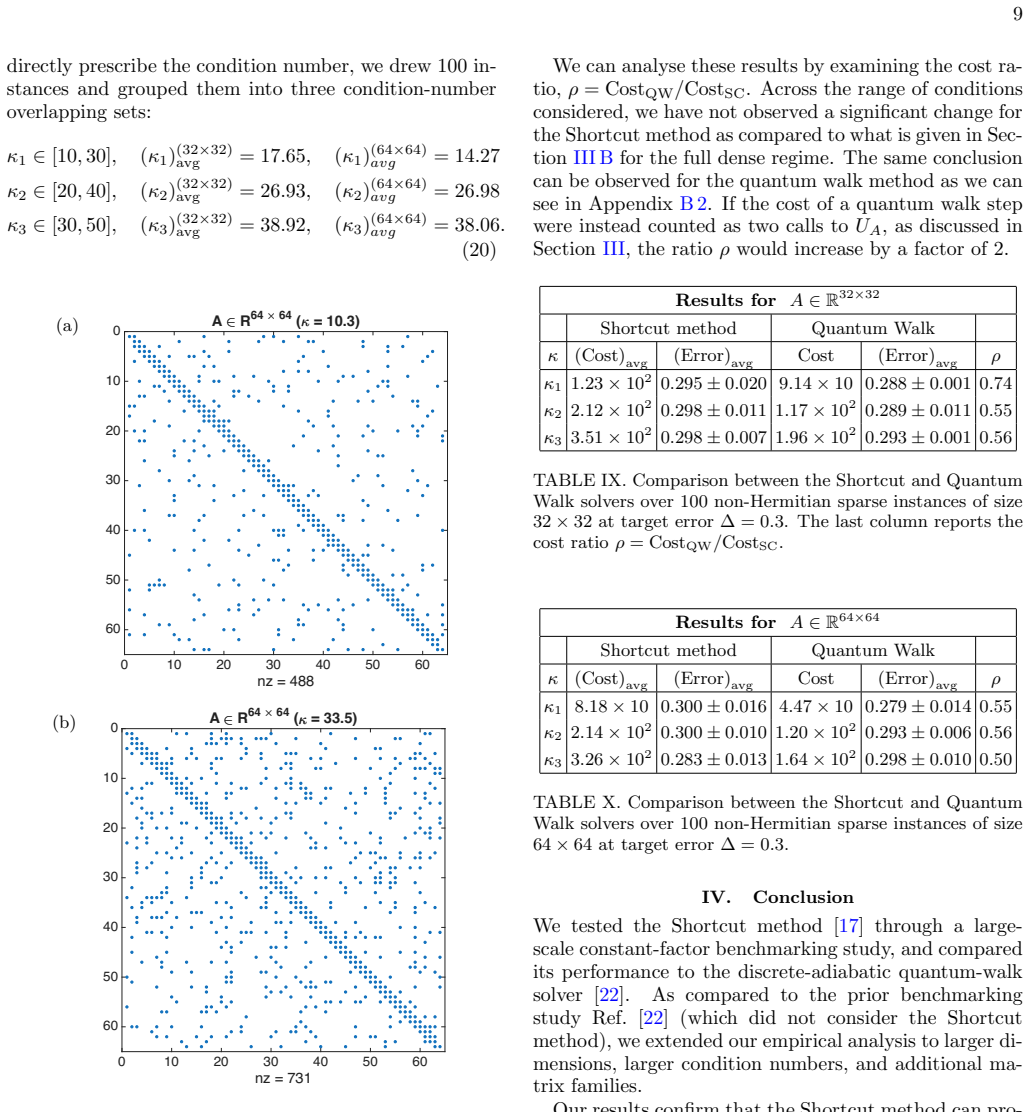
Non-Hermitian matrices Rather than selecting a distinct value of ηKR for each matrix instance to meet the target error, we determine a single global value ofηKR for all instances associated with a fixed condition number. This global ηKR is chosen such that the average error across all 100 non-Hermitian ma- trix samples matches the desired target threshold...
-
[6]
ex- haustive search in log space
Positive definite matrices We next test the Shortcut method on positive-definite matrices with a known solution norm. For these in- stances, the QW method is known to have a substan- tially smaller constant factor than in the non-Hermitian TABLE IV. Shortcut method performance for ϵ = 0 .001 on A ∈ R64×64, averaged over 100 non-Hermitian instances. For ea...
-
[7]
Quantum Linear System Solvers: A Survey of Algorithms and Applications
M. Morales, L. Pira, P. Schleich, K. Koor, P. Costa, D. An, A. Aspuru-Guzik, L. Lin, P. Rebentrost, and D. Berry, arXiv:2411.02522 (2024)
-
[8]
D. W. Berry and P. C. S. Costa, Quantum8, 1369 (2024)
2024
-
[9]
P. C. Costa, P. Schleich, M. E. Morales, and D. W. Berry, npj Quantum Information 11, 141 (2025)
2025
-
[10]
J.-P. Liu, D. An, D. Fang, J. Wang, G. H. Low, and S. Jordan, Communications in Mathematical Physics 404, 963 (2023)
2023
-
[11]
H. Zhao, A. Zlokapa, H. Neven, R. Babbush, J. Preskill, J. R. McClean, and H.-Y. Huang, arXiv:2604.07639 (2026)
work page internal anchor Pith review Pith/arXiv arXiv 2026
-
[12]
A. W. Harrow, A. Hassidim, and S. Lloyd, Physical Re- view Letters 103, 150502 (2009)
2009
-
[13]
Ambainis (Schloss Dagstuhl – Leibniz-Zentrum f¨ ur In- formatik, 2012) pp
A. Ambainis (Schloss Dagstuhl – Leibniz-Zentrum f¨ ur In- formatik, 2012) pp. 636–647
2012
-
[14]
A. Ambainis, arXiv:1010.4458 (2010)
-
[15]
A. M. Childs, R. Kothari, and R. D. Somma, SIAM Journal on Computing 46, 1920 (2017)
1920
-
[16]
Suba¸ sı, R
Y. Suba¸ sı, R. D. Somma, and D. Orsucci, Physical Re- view Letters 122, 060504 (2019)
2019
-
[17]
An and L
D. An and L. Lin, ACM Transactions on Quantum Com- puting 3, 5 (2022)
2022
-
[18]
Lin and Y
L. Lin and Y. Tong, Quantum 4, 361 (2020)
2020
-
[19]
P. C. Costa, D. An, Y. R. Sanders, Y. Su, R. Babbush, and D. W. Berry, PRX Quantum 3, 040303 (2022)
2022
-
[20]
D. Jennings, M. Lostaglio, S. Pallister, A. T. Sornborger, and Y. Suba¸ sı, arXiv:2305.11352 (2023)
-
[21]
Cunningham and J
J. Cunningham and J. Roland (Schloss Dagstuhl – Leibniz-Zentrum f¨ ur Informatik, 2024) pp. 7:1–7:20
2024
-
[22]
Jennings, M
D. Jennings, M. Lostaglio, S. Pallister, A. T. Sornborger, and Y. Suba¸ sı, PRX Quantum6, 040373 (2025)
2025
-
[23]
A. M. Dalzell, arXiv:2406.12086 (2024)
work page internal anchor Pith review Pith/arXiv arXiv 2024
-
[24]
A. M. Dalzell, B. D. Clader, G. Salton, M. Berta, C. Y.- Y. Lin, D. A. Bader, N. Stamatopoulos, M. J. A. Schuetz, F. G. S. L. Brand˜ ao, H. G. Katzgraber, and W. J. Zeng, PRX Quantum 4, 040325 (2023)
2023
-
[25]
Jennings, M
D. Jennings, M. Lostaglio, R. B. Lowrie, S. Pallister, and A. T. Sornborger, Quantum 8, 1553 (2024)
2024
- [26]
-
[27]
D. Jennings, K. Korzekwa, M. Lostaglio, R. Ashworth, E. Marsili, and S. Rolston, arXiv:2512.03758 (2025)
-
[28]
P. C. S. Costa, D. An, R. Babbush, and D. W. Berry, Quantum 9, 1887 (2025)
2025
-
[29]
Gily´ en, Y
A. Gily´ en, Y. Su, G. H. Low, and N. Wiebe, in Proceed- ings of the 51st Annual ACM SIGACT Symposium on Theory of Computing (2019) pp. 193–204
2019
-
[30]
QLSP—Shortcut method: Quan- tum linear systems problem solver and sparse- matrix generator,
P. C. S. Costa, “QLSP—Shortcut method: Quan- tum linear systems problem solver and sparse- matrix generator,” https://github.com/PcostaQuantum/ QLSP---Shortcut-method (2025), gitHub repository; ac- cessed 2025-09-04. A. The kernel reflection and the kernel projection The algorithm that we will be focusing on here is based on the kernel projection (KP) and...
2025
-
[31]
Kernel Projection The KP takes two parameters (ηKP, κ) and only works under the promise that the nonzero singular values of G lie in the interval [κ−1, 1] which we already showed that is the case. Let us consider an arbitrary normalized s-qubit state |ϕ⟩ = γ |w⟩+ν |w⊥⟩, where w is a unit vector in the kernel of G, which typically for us it will be |w⟩ = |...
-
[32]
For all x ∈ [−1, 1], it holds that |F e∆,l(x)| ≤ 1
-
[33]
For all x ∈ [e∆, 1], it holds that |F e∆,l(x)| ≤ Tl 1+ e∆2 1− e∆2 −1 ≤ ηKP
-
[34]
F e∆,l(0) = 1. The properties outlined above indicate that F e∆,l(x) func- tions as a filter with width e∆, mapping the zero input to one and assigning values close to zero for all inputs out- side the interval [−e∆,e∆]. The idea is to apply the QSVT using the polynomial F e∆,t. Following the example provided by [17], we consider a more detailed explanati...
-
[35]
Lemma 1 (Using KP to refine QLSS solution)
following its proof. Lemma 1 (Using KP to refine QLSS solution). Suppose b is in the column space of A, and let x denote the so- lution of minimum ∥x∥ to the equation Ax = b. Suppose A has no singular values in the interval 0, κ−1 and let ˜ρ be a mixed quantum state for which ⟨x| ˜ρ |x⟩ = 1 − µ2 and ⟨y| ˜ρ |y⟩ that are in the kernel of A. Suppose KP is ap...
-
[36]
The ηKR parameter plays the same role as ηKP but may be chosen to take a different value
Kernel Reflection The KR also takes the two input parameters ( ηKR, κ). The ηKR parameter plays the same role as ηKP but may be chosen to take a different value. We choose l as in Eq. (A16), with ηKR in place of ηKP. KR maps the quan- tum state |ϕ⟩ = γ |w⟩ + ν |w⊥⟩ as follows γ |w⟩ + ν |w⊥⟩ → γ |w⟩ − ν(1 − δ′
-
[37]
|w⊥⟩ + νδ ′ 2 |w′ ⊥⟩ , (A26) which are the same vectors given in Eq. (A10), where δ′ 1 = 2(ηKR + δ1) 1 + ηKR , δ ′ 2 = 2δ2 1 + ηKR , (A27) from where the following relations can be derived δ′ 1 ≥ 0, q δ′2 1 + δ′2 2 ≤ 4ηKR 1 + ηKR , |δ′ 2| ≤ 2ηKR 1 + ηKR . (A28) Similarly to the KP we can build a 2 l-degree polyno- mial within the framework of QSVT for the...
-
[38]
For all x ∈ [−1, 1], it holds that |K e∆,l(x)| ≤ 1. (A30)
-
[39]
For all x ∈ [e∆, 1], it holds that |K e∆,l(x)| ≤ − 1 + 4 Tl 1+ e∆2 1− e∆2 + 1 ≤ −1 + 4ηKR 1 + ηKR . (A31)
-
[40]
Now let us do the same exercise that we have done for KP
K e∆,l(0) = 1. Now let us do the same exercise that we have done for KP. We consider the state |ϕ⟩ = c1 |a⟩ + c2 |b⟩ where a is a vector in the kernel of H, and b is orthogonal to the kernel. We again assume that the vector |b⟩ has the following decompositionP j wj |uj⟩. We now look at the action of the polynomial K e∆,l of the matrix H, so in this case w...
-
[41]
(A34) We also known from the properties of F e∆,t(x) that for all x ∈ [e∆, 1], ηKR ≥ | F e∆,l(x)|, so if we consider |F e∆,l(e∆)| = ηKR we recover Eq
|b⟩ + δ′ 2 |b′⟩ , (A33) where δ′ 1 = 2F e∆,l(e∆) + 2δ1 1 + F e∆,l(e∆) , δ ′ 2 = 2δ2 1 + F e∆,l(e∆) . (A34) We also known from the properties of F e∆,t(x) that for all x ∈ [e∆, 1], ηKR ≥ | F e∆,l(x)|, so if we consider |F e∆,l(e∆)| = ηKR we recover Eq. (A27). Finally, we can conclude U(H) K e∆,l |0⟩⊗(aH+1) ⊗ |ϕ⟩ = |0⟩⊗(aH+1) ⊗ (c1 |a⟩ −c2(1 − δ′
-
[42]
|b⟩ + c2δ′ 2 |b′⟩) + c2 q 2δ′ 1 − δ ′2 1 − δ ′2 2 |⊥⟩ . (A35)
-
[43]
Comparison to QW filtering and double cost There are a number of subtleties in comparing the cost of the QSVT filter for the KP in the Shortcut method versus the filter used for the QW in Ref. [22]. For the KP of the Shortcut method, there is a factor of 1 /2 in Eq. (A16), which is not present in Eq. (113) of Ref. [22]. However, the degree of the polynomi...
-
[44]
We tested both approaches, considering different dimensions across different condition numbers
for the QW and the Randomised method. We tested both approaches, considering different dimensions across different condition numbers. Moreover, we give the plots for the recommended values for ∆ accordingly to a given target precision for ϵ for the solution error for both meth- ods, i.e., QW and Shortcut for the non-Hermitian matri- ces
-
[45]
We also provide the corresponding tables for the positive- definite (PD) cases
Recommended values for ∆ We begin by presenting the results for the QW method applied to non-Hermitian matrices, including the tables used to interpolate the cost values as a function of ∆. We also provide the corresponding tables for the positive- definite (PD) cases. These results then allow us to de- termine the recommended values of ∆ that minimize th...
-
[46]
Extended analysis of the QW and Randomised method We report the results over 100 instances by fixing the walk step, in the QW method, so we get on average the following set of δ values: ∆ ∈ { 0.4, 0.3, 0.25, 0.20, 0.15}, which is reported in Tables B.I, B.II and B.VII to B.IX, which represents the costly part of the quantum linear solvers, accordingly to ...
2072
discussion (0)
Sign in with ORCID, Apple, or X to comment. Anyone can read and Pith papers without signing in.