Recognition: unknown
Analytical and Compressed Simulation of Noisy Stabilizer Circuits
Pith reviewed 2026-05-08 12:03 UTC · model grok-4.3
The pith
Closed-form expressions for Pauli expectations enable efficient strong simulation of noisy stabilizer circuits without constructing density matrices.
A machine-rendered reading of the paper's core claim, the machinery that carries it, and where it could break.
Core claim
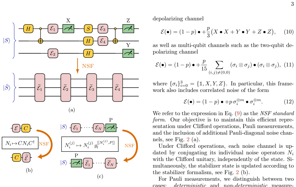
Closed-form expressions of expectation values for tensor products of Paulis are derived for circuits containing non-deterministic Pauli measurements; these expressions furnish an efficient strong simulation method that never builds the full density matrix and permits immediate noise-parameter sweeps. A circuit-compression framework further reduces the per-sample cost of weak simulation for general noisy stabilizer circuits by separating parameter-independent preprocessing from sampling. The analytical reach is extended to include a small number of deterministic measurements, general rotations, and non-diagonal noise channels, producing a single framework for both strong and weak simulation.
What carries the argument
Closed-form expressions for Pauli-tensor expectation values together with a circuit-compression procedure that isolates preprocessing from sampling.
If this is right
- Expectation values of entanglement witnesses can be obtained directly from the closed forms.
- Reduced density matrices of subsystems follow from the same analytic expressions.
- Energy evaluation in noisy quantum systems becomes feasible by sweeping noise parameters without repeated full simulations.
- Weak simulation cost drops because preprocessing is performed once per circuit topology.
- The formalism now covers limited deterministic measurements and non-diagonal noise while retaining efficiency.
Where Pith is reading between the lines
- The preprocessing separation could be reused to accelerate Monte-Carlo sampling in other circuit families that admit partial analytic treatment.
- Direct noise-parameter sweeps enable gradient-based optimization of noise levels inside variational algorithms that remain approximately stabilizer.
- If the limited extensions to deterministic measurements scale, hybrid protocols mixing a few non-Clifford gates with many stabilizer operations may still admit efficient partial simulation.
Load-bearing premise
Noise channels and measurement outcomes stay inside the stabilizer formalism so that the closed-form expressions and compression rules continue to apply without further approximations.
What would settle it
Exact numerical computation of Pauli expectations on a small circuit containing a non-stabilizer noise channel or measurement whose outcome lies outside the stabilizer group would differ from the closed-form prediction.
Figures


read the original abstract
We develop analytical and algorithmic techniques that enable efficient simulation of a broad class of noisy stabilizer circuits. We derive closed-form expressions of expectation values for tensor product of Paulis in circuits with non-deterministic Pauli measurements, yielding an efficient strong simulation method that avoids explicit density matrix construction and enables direct noise parameter sweeps. We introduce a circuit compression framework that reduces the per-sample cost of weak simulation in general noisy stabilizer circuits, including deterministic measurements, by separating parameter-independent preprocessing from sampling. Finally, we extend the analytical framework beyond its standard domain to include a small number of deterministic measurements, general rotations, and non-diagonal noise channels. Our results provide a unified framework for both strong and weak simulation of noisy stabilizer circuits and corresponds to an extension of the noisy stabilizer formalism introduced in \cite{PhysRevA.107.032424}. They offer applications ranging from calculation of the expectation values of entanglement witnesses, determination of reduced states, to energy evaluation.
Editorial analysis
A structured set of objections, weighed in public.
Referee Report
Summary. The manuscript develops analytical and algorithmic methods for efficient simulation of noisy stabilizer circuits. It derives closed-form expressions for expectation values of Pauli tensor products in the presence of non-deterministic Pauli measurements, enabling strong simulation that avoids explicit density-matrix construction and supports direct noise-parameter sweeps. A circuit-compression framework is introduced to reduce per-sample cost for weak simulation of general noisy stabilizer circuits (including deterministic measurements) by separating parameter-independent preprocessing from sampling. The work extends the analytical framework to a limited number of deterministic measurements, general rotations, and non-diagonal noise channels, and positions the results as an extension of the noisy stabilizer formalism of PhysRevA.107.032424 with applications to entanglement witnesses, reduced states, and energy evaluation.
Significance. If the closed-form expressions and compression rules are rigorously derived and verified, the results would offer a practical advance in strong and weak simulation of noisy Clifford circuits, particularly for parameter sweeps and moderate-depth circuits where explicit density-matrix methods become prohibitive. The separation of preprocessing from sampling and the explicit handling of non-deterministic measurements address a common bottleneck in stabilizer-based noise analysis. The limited-scope extensions to deterministic measurements and non-diagonal channels are useful but do not claim universality.
major comments (3)
- [§3] §3 (Closed-form derivation): The claim that the expectation-value expressions remain closed-form and parameter-free for non-deterministic Pauli measurements must be verified against the explicit formulas; if the derivation invokes the stabilizer subspace closure property only for diagonal noise, the extension to non-diagonal channels (mentioned in the abstract) requires an explicit statement of the additional assumptions or truncation that preserves the closed form.
- [§4] §4 (Compression framework): The per-sample cost reduction for weak simulation is stated to arise from separating preprocessing from sampling, but the manuscript does not quantify the scaling with the number of deterministic measurements; if even a modest number (e.g., >5) forces explicit summation over 2^k branches, the claimed efficiency advantage for general circuits is not load-bearing.
- [§5] §5 (Extension to deterministic measurements and non-diagonal noise): The abstract qualifies the extension as applying to “a small number” of deterministic measurements; the manuscript should provide a concrete bound or scaling result showing when the closed-form property is lost, otherwise the central efficiency claim for the extended regime rests on an unstated regime restriction.
minor comments (3)
- Notation for the noise channels (e.g., the definition of the non-diagonal Kraus operators) is introduced without a dedicated table or appendix; a compact summary table would improve readability.
- The abstract cites PhysRevA.107.032424 but the introduction does not explicitly delineate which results are reproduced versus newly derived; a short “relation to prior work” paragraph would clarify novelty.
- Figure captions for the numerical benchmarks should state the circuit depth, number of qubits, and noise strength ranges used, rather than leaving these details only in the text.
Simulated Author's Rebuttal
We thank the referee for the careful reading of our manuscript and the constructive comments. We address each major comment below and will make the corresponding revisions to clarify the scope and strengthen the presentation.
read point-by-point responses
-
Referee: [§3] §3 (Closed-form derivation): The claim that the expectation-value expressions remain closed-form and parameter-free for non-deterministic Pauli measurements must be verified against the explicit formulas; if the derivation invokes the stabilizer subspace closure property only for diagonal noise, the extension to non-diagonal channels (mentioned in the abstract) requires an explicit statement of the additional assumptions or truncation that preserves the closed form.
Authors: We thank the referee for this observation. The closed-form expressions derived in Section 3 follow from the action of Pauli measurements on the stabilizer subspace and are explicitly parameter-free for non-deterministic measurements; the formulas are obtained by direct algebraic manipulation without summation over outcomes. The derivation relies on the stabilizer closure property, which holds for the Pauli noise model considered. For the extension to non-diagonal channels, the framework applies when the noise admits a Pauli decomposition or when off-diagonal contributions are averaged over the stabilizer group; we will add an explicit statement of these assumptions in Section 3 and the abstract to remove any ambiguity. revision: yes
-
Referee: [§4] §4 (Compression framework): The per-sample cost reduction for weak simulation is stated to arise from separating preprocessing from sampling, but the manuscript does not quantify the scaling with the number of deterministic measurements; if even a modest number (e.g., >5) forces explicit summation over 2^k branches, the claimed efficiency advantage for general circuits is not load-bearing.
Authors: We appreciate the referee highlighting the need for explicit scaling. The compression in Section 4 precomputes all parameter-independent circuit elements once, after which each sample only requires evaluating the compressed representation. For deterministic measurements the cost scales as O(2^k poly(n)) for the initial compression step when k such measurements are present, but the per-sample cost remains O(poly(n)) thereafter. We will add a quantitative discussion of this scaling in Section 4, emphasizing that the method targets the regime of small k (as qualified in Section 5) where the advantage over full density-matrix simulation is retained. revision: yes
-
Referee: [§5] §5 (Extension to deterministic measurements and non-diagonal noise): The abstract qualifies the extension as applying to “a small number” of deterministic measurements; the manuscript should provide a concrete bound or scaling result showing when the closed-form property is lost, otherwise the central efficiency claim for the extended regime rests on an unstated regime restriction.
Authors: We agree that a concrete bound improves clarity. The phrase “small number” in the abstract and Section 5 is meant to indicate that k remains constant or grows at most logarithmically with n so that the 2^k factor does not dominate. We will revise Section 5 to state an explicit practical bound (e.g., k ≤ 8 for n ≈ 100) together with the scaling relation showing when the closed-form expressions transition to explicit enumeration, thereby making the regime of applicability precise. revision: yes
Circularity Check
No significant circularity; derivations rest on standard stabilizer algebra and explicit analytical steps
full rationale
The paper's core contribution consists of deriving closed-form expressions for Pauli expectation values under non-deterministic measurements by direct manipulation within the stabilizer formalism, followed by a compression framework that separates preprocessing from sampling. These steps are presented as analytical extensions rather than reductions to fitted parameters, self-referential definitions, or load-bearing self-citations that presuppose the target results. The single reference to the prior noisy stabilizer formalism (PhysRevA.107.032424) serves as background context for the extension and does not substitute for the new closed-form derivations or compression rules, which remain independently verifiable from the circuit structure and noise model assumptions stated in the manuscript.
Axiom & Free-Parameter Ledger
axioms (1)
- standard math Standard properties of stabilizer circuits and Pauli operators hold under the given noise models
Reference graph
Works this paper leans on
-
[1]
A first key difference is their information content
Deterministic versus non-deterministic measurements Here, we highlight the key differences between deter- ministic and non-deterministic Pauli measurements in noisy stabilizer circuits and connect them to the NSF. A first key difference is their information content. For non-deterministic measurements, the outcomes re- main uniformly distributed over±1, ev...
-
[2]
A stabilizer tableau simulator represents ann-qubit stabilizer state using a binary data structure that tracks a generating set of the stabilizer group under Clifford evo- lution
Stabilizer tableau As a first step, we introduce the concept of a stabilizer tableau, which is utilized to efficiently store and update a noiseless stabilizer state, under Pauli measurements and Clifford gates. A stabilizer tableau simulator represents ann-qubit stabilizer state using a binary data structure that tracks a generating set of the stabilizer ...
-
[3]
The central idea is to separate the simulation into two components: (1) a noiseless reference trajectory and (2) classically tracked Pauli errors (the Pauli frame)
Pauli frame sampling Pauli-frame simulation [7] is a technique to efficiently generate large numbers of samples from noisy stabilizer circuits without re-running a full tableau simulation for every shot. The central idea is to separate the simulation into two components: (1) a noiseless reference trajectory and (2) classically tracked Pauli errors (the Pa...
-
[4]
Each qubit therefore carries two bits(xi, zi)
Pauli Frames A Pauli frame is a classical record specifying, for each qubit, whether the current state differs from a reference state by anXand/orZoperator. Each qubit therefore carries two bits(xi, zi). Clifford gates update the frame by conjugation, which acts as a deterministic linear trans- formationonthebits(x i, zi). Thisupdateischeaperthan evolving...
-
[5]
Instead, at each noise location a Pauli operator is sampled from the channel distribution and multiplied into the Pauli frame
Noise Accumulation For Pauli channels, one does not apply noise directly to the stabilizer state. Instead, at each noise location a Pauli operator is sampled from the channel distribution and multiplied into the Pauli frame
-
[6]
Therefore, one first computes a noiseless reference shot using a stabilizer tableau simu- lator
Reference Sample and Outcome Generation APauli-framesimulatoryieldsonlytheparityflipsthat should be applied to measurement outcomes, where the measurements are restricted without loss of generality to Pauli-Zmeasurements. Therefore, one first computes a noiseless reference shot using a stabilizer tableau simu- lator. For each subsequently sampled Pauli fr...
-
[7]
For stabilizer and graph states, witnesses can be constructed directly from stabi- lizer generators
Entanglement witnesses Entanglement witnesses [24] provide operational crite- ria to detect non-separability. For stabilizer and graph states, witnesses can be constructed directly from stabi- lizer generators. For example, bipartite and multipartite entanglement witnesses can be constructed as W=1− X i cigi,(26) whereg i are stabilizer generators andci ∈...
-
[8]
Reduced density matrices and local entropies Any reduced density matrix on a subsystemAcan be reconstructed by restricting the stabilizer expansion to operators supported onA, ρA = 1 2|A| X Sl∈S: supp(Sl)⊆A ⟨Sl⟩Sl.(28) Hence,ρ A can be determined efficiently and analytically from the2 |A| Pauli expectation values using the methods of Sec. IIIA. Pure stabi...
-
[9]
Bell inequality violations Bell-type inequalities consider an-partite scenario in which partyichooses one of two dichotomic observables, A(i) xi withx i ∈ {0,1}, each producing outcomes±1. The resulting correlations are described by the correlators D A(i1) xi1 · · ·A (ik) xik E ρ .(29) In this setting, a general Bell-type inequality takes the form nX k=1 ...
-
[10]
This assumption is not very restrictive
Energy expectation values of Hamiltonians ForHamiltoniansthatcanbewrittenasapoly(n)-term sum of Pauli operators, ⟨H⟩ ρ = X i hi⟨Pi⟩,(31) whereh i ∈R, the energy can be computed directly from poly(n)Pauli expectation values. This assumption is not very restrictive. Anyn-qubit Hamiltonian with only fi- nitek-body interactions can be expanded in the Pauli ba...
-
[11]
ArecentlyintroducedqualitymetricfornoisyMBQCis the average MBQC fidelity [34]
Average MBQC fidelity. ArecentlyintroducedqualitymetricfornoisyMBQCis the average MBQC fidelity [34]. Rather than evaluating the fidelity of the full resource state, one fixes the out- put vertices and averages over all measurement angles, yielding F MBQC(ρ). This quantity admits the compact form F MBQC(ρ) = tr(ρΩ),(33) whereΩis a weighted sum of stabiliz...
-
[12]
We consider cater- pillars with two leaves at each linear cluster vertex, and when fusing two caterpillar graph states, we fuse always one leaf per node, see Fig
Fusion of noisy caterpillar states We consider the fusion of caterpillar graph states, whichisalinearclustergraphstatewithacertainnumber of leaves at each linear cluster vertex. We consider cater- pillars with two leaves at each linear cluster vertex, and when fusing two caterpillar graph states, we fuse always one leaf per node, see Fig. 4 for an illustr...
-
[13]
Nowwe con- sider the case where the operations are noisy, as well as analyze the noisy generation process of the noisy cater- pillar graph states
Noisy generation and fusion of caterpillar states with imperfect operations The analysis above, demonstrates the effect of initial noise beingtransformedbyideal operations. Nowwe con- sider the case where the operations are noisy, as well as analyze the noisy generation process of the noisy cater- pillar graph states. We model noisy one qubit gates by an ...
-
[14]
The random measurement observableP0 commutes with all measurement blocks
-
[15]
(47), for some t∈F n 2
The random measurement observableP 0 = dα0 1 1 · · ·d α0 n n gβ0 1 1 · · ·g β0 n n and the random measurement observables contained in the measurement blocks Pj =d αj 1 1 · · ·d αj n n g βj 1 1 · · ·g βj n n fulfill Eq. (47), for some t∈F n 2. If those conditions are not fulfilled the random measure- ment cannot be absorbed and has to be appended. These r...
-
[16]
Methodology Deterministic measurements occur when the measure- ment observable is contained in the stabilizer group, i.e., P≡S l ∈ S. The post-measurement state can then be written as ρ′ ∝ 1±S l 2| {z } ≡PSl ,± E1 · · · EN(|S⟩ ⟨S|)| {z } ≡ρ 1±S l 2 .(49) Note thatρ ′ is only proportional to the action of the projector, since normalization by the probabili...
-
[17]
Deterministic measurements Fordeterministicmeasurementswithrespecttotheref- erence stabilizer state, we run into the same issue as in the standard NSF framework. We cannot make the mea- surement operator commuting with the noise channels. Hence, if we propagate the measurement to the state, we will expand the measurement operator analogous to thedetermini...
-
[18]
M. F. Mor-Ruiz and W. Dür, Phys. Rev. A107, 032424 (2023)
2023
-
[19]
Villalonga, S
B. Villalonga, S. Boixo, B. Nelson, C. Henze, E. Rieffel, R. Biswas, and S. Mandrà, npj Quantum Information5, 86 (2019)
2019
-
[20]
Aaronson and D
S. Aaronson and D. Gottesman, Physical Review A—Atomic, Molecular, and Optical Physics70, 052328 (2004)
2004
-
[21]
Gidney, Quantum5, 497 (2021)
C. Gidney, Quantum5, 497 (2021)
2021
-
[22]
Gottesman,The Heisenberg Representation of Quan- tum Computers, Tech
D. Gottesman,The Heisenberg Representation of Quan- tum Computers, Tech. Rep. LA-UR-98-2848; CONF- 980788- (Los Alamos National Laboratory, Los Alamos, NM, 1998)
1998
-
[23]
Anders and H
S. Anders and H. J. Briegel, Phys. Rev. A73, 022334 (2006)
2006
-
[24]
P. Rall, D. Liang, J. Cook, and W. Kretschmer, Phys. Rev. A99, 062337 (2019)
2019
-
[25]
M. A. Nielsen and I. L. Chuang,Quantum Computa- tion and Quantum Information: 10th Anniversary Edi- tion(Cambridge University Press, Cambridge, 2010)
2010
-
[26]
M. F. Mor-Ruiz, J. Wallnöfer, and W. Dür, Quantum9, 1605 (2025)
2025
-
[27]
M. F. Mor-Ruiz and W. Dür, IEEE Journal on Selected Areas in Communications42, 1793 (2024)
2024
-
[28]
Merging-based quantum repeater,
M. F. Mor-Ruiz, J. Miguel-Ramiro, J. Wallnöfer, T. Coopmans, and W. Dür, “Merging-based quantum repeater,” (2025), arXiv:2502.04450 [quant-ph]
-
[29]
Aigner, M
P. Aigner, M. F. Mor-Ruiz, and W. Dür, Phys. Rev. A 112, 022402 (2025)
2025
-
[30]
Raussendorf and H
R. Raussendorf and H. J. Briegel, Phys. Rev. Lett.86, 5188 (2001)
2001
-
[31]
Freund, A
J. Freund, A. Pirker, L. Vandré, and W. Dür, New Jour- nal of Physics27, 094505 (2025)
2025
-
[32]
Szymański, L
K. Szymański, L. Vandré, and O. Gühne, Quantum10, 1977 (2026)
1977
-
[33]
Improved routing of multi- party entanglement over quantum networks,
N. Basak and G. Paul, “Improved routing of multi- party entanglement over quantum networks,” (2024), arXiv:2409.14694 [quant-ph]
-
[34]
A. Sen, K. Goodenough, and D. Towsley, Quantum9, 1911 (2025)
1911
-
[35]
A. Dahlberg and S. Wehner, Philosophical Trans- actions of the Royal Society A: Mathematical, Physical and Engineering Sciences376, 20170325 (2018), https://royalsocietypublishing.org/rsta/article- pdf/doi/10.1098/rsta.2017.0325/1401018/rsta.2017.0325.pdf
work page doi:10.1098/rsta.2017.0325/1401018/rsta.2017.0325.pdf 2018
-
[36]
Van den Nest, J
M. Van den Nest, J. Dehaene, and B. De Moor, Phys. Rev. A69, 022316 (2004)
2004
- [37]
-
[38]
N. Brandl, M. Cherniak, J. Kofler, and R. Kueng, “Quickqudits: A framework for efficient simulation of noisy qudit clifford circuits via an extended stabilizer tableauformalism,” (2026),arXiv:2603.23641[quant-ph]
-
[39]
Sdim: A qudit stabilizer simulator,
A. Kabir, S. Nguyen, S. Ghosh, T. Kiran, I. H. Kim, and Y. Huang, “Sdim: A qudit stabilizer simulator,” (2025), arXiv:2511.12777 [quant-ph]
work page internal anchor Pith review arXiv 2025
-
[40]
LightStim: A Framework for QEC Protocol Evaluation and Prototyping with Automated DEM Construction
X. Fang, M. Wang, Y. Wu, S. Prabhu, D. Tullsen, N. R. Miniskar, F. Mueller, T. Humble, and Y. Ding, “Light- stim: A framework for qec protocol evaluation and pro- totyping with automated dem construction,” (2026), arXiv:2604.21472 [quant-ph]
work page internal anchor Pith review Pith/arXiv arXiv 2026
-
[41]
Gühne and G
O. Gühne and G. Tóth, Physics Reports474, 1 (2009)
2009
-
[42]
Tóth and O
G. Tóth and O. Gühne, Phys. Rev. A72, 022340 (2005)
2005
-
[43]
N. K. H. Li, X. Dai, M. H. Muñoz-Arias, K. Reuer, M. Huber, and N. Friis, Nature Communications17, 1707 (2026)
2026
-
[44]
Wu, Y.-h
X. Wu, Y.-h. Yang, Y.-k. Wang, Q.-y. Wen, S.-j. Qin, and F. Gao, Phys. Rev. A92, 012305 (2015)
2015
-
[45]
F. Shi, L. Chen, G. Chiribella, and Q. Zhao, Phys. Rev. Lett.134, 050201 (2025)
2025
-
[46]
Quantum state determinability from local marginals is universally robust
W. Yu, F. Shi, G. Chiribella, and Q. Zhao, “Quantum state determinability from local marginals is universally robust,” (2026), arXiv:2604.05508 [quant-ph]
work page internal anchor Pith review Pith/arXiv arXiv 2026
-
[47]
M. B. Ruskai, Journal of Mathematical Physics43, 4358 (2002)
2002
-
[48]
Gühne, G
O. Gühne, G. Tóth, P. Hyllus, and H. J. Briegel, Phys. Rev. Lett.95, 120405 (2005)
2005
-
[49]
Baccari, R
F. Baccari, R. Augusiak, I. Šupić, J. Tura, and A. Acín, Phys. Rev. Lett.124, 020402 (2020)
2020
-
[50]
J. Sun, L. Cheng, and S.-X. Zhang, Quantum9, 1782 (2025)
2025
-
[51]
Directly estimating the fidelity of measurement-based quantum computation,
D. T. Stephen and M. Foss-Feig, “Directly estimating the fidelity of measurement-based quantum computation,” (2026), arXiv:2603.13753v1, 2603.13753
-
[52]
S. T. Flammia and Y.-K. Liu, Phys. Rev. Lett.106, 230501 (2011)
2011
-
[53]
Monte carlo theory, methods and exam- ples,
A. B. Owen, “Monte carlo theory, methods and exam- ples,” (2013)
2013
-
[54]
Hoeffding, Journal of the American Statistical Asso- ciation58, 13 (1963)
W. Hoeffding, Journal of the American Statistical Asso- ciation58, 13 (1963)
1963
-
[55]
M. Hein, J. Eisert, and H. J. Briegel, Phys. Rev. A69, 062311 (2004)
2004
-
[56]
Enrico Fermi
M. Hein, W. Dür, J. Eisert, R. Raussendorf, M. Van den Nest, and H. J. Briegel, inQuantum Computers, Al- gorithms and Chaos, Proceedings of the International School of Physics “Enrico Fermi”, Vol. 162, edited by G. Casati, D. L. Shepelyansky, P. Zoller, and G. Benenti (IOS Press, 2006) pp. 115–218
2006
-
[57]
Bartolucci, P
S. Bartolucci, P. Birchall, H. Bombín, H. Cable, C. Daw- son, M. Gimeno-Segovia, E. Johnston, K. Kieling, N. Nickerson, M. Pant, F. Pastawski, T. Rudolph, and C. Sparrow, Nature Communications14, 912 (2023)
2023
-
[58]
M. C. Löbl, L. A. Pettersson, A. Jena, L. Dellantonio, S.Paesani, andA.S.Sørensen,Phys.Rev.A111,052604 (2025)
2025
-
[59]
Noisy graph states 0.4,
J. Wallnöfer and M. F. Mor-Ruiz, “Noisy graph states 0.4,” (2025)
2025
-
[60]
Pirker, J
A. Pirker, J. Wallnöfer, and W. Dür, New Journal of Physics20, 053054 (2018)
2018
-
[61]
Kruszynska, A
C. Kruszynska, A. Miyake, H. J. Briegel, and W. Dür, Phys. Rev. A74, 052316 (2006)
2006
-
[62]
N. H. Lindner and T. Rudolph, Physical Review Letters 103, 113602 (2009)
2009
-
[63]
Thomas, L
P. Thomas, L. Ruscio, O. Morin, and G. Rempe, Nature 608, 677 (2022). 15
2022
-
[64]
D. E. Browne and T. Rudolph, Phys. Rev. Lett.95, 010501 (2005)
2005
-
[65]
Lee and H
S.-H. Lee and H. Jeong, Quantum7, 1212 (2023)
2023
-
[66]
M. C. Löbl, S. Paesani, and A. S. Sørensen, Quantum8, 1302 (2024)
2024
-
[67]
2019, Contemporary Physics, 60, 111, doi: 10.1080/00107514.2019.1615715
J. Roffe, Contemporary Physics60, 226 (2019), https://doi.org/10.1080/00107514.2019.1667078
-
[68]
Dür and H
W. Dür and H. J. Briegel, Reports on Progress in Physics 70, 1381 (2007)
2007
-
[69]
Matti,Extensions and Limitations of the Noisy Stabi- lizer Formalism, Master’s thesis, University of Innsbruck, Innsbruck (2025)
J. Matti,Extensions and Limitations of the Noisy Stabi- lizer Formalism, Master’s thesis, University of Innsbruck, Innsbruck (2025)
2025
-
[70]
A100, 052333 (2019)
C.Meignant, D.Markham, andF.Grosshans,Phys.Rev. A100, 052333 (2019)
2019
-
[71]
SyQMA: A memory-efficient, symbolic and exact universal simulator for quantum error correction
G. Umbrarescu and D. Amaro, “Syqma: A memory- efficient, symbolic and exact universal simulator for quan- tum error correction,” (2026), arXiv:2604.15043 [quant- ph]
work page internal anchor Pith review Pith/arXiv arXiv 2026
-
[72]
noisy_stabilizers_d,
qcomm-uibk, “noisy_stabilizers_d,” GitHub repository
-
[73]
Gutiérrez, L
M. Gutiérrez, L. Svec, A. Vargo, and K. R. Brown, Phys. Rev. A87, 030302 (2013)
2013
-
[74]
Magesan, D
E. Magesan, D. Puzzuoli, C. E. Granade, and D. G. Cory, Phys. Rev. A87, 012324 (2013). Appendix A: Numerical complexity of the NSF We analyze the numerical complexity of updating noise channels within the NSF framework. Since different noise channels can be updated independently, these updates can be parallelized. Therefore, it suffices to analyze the com...
2013
-
[75]
One, can reduce the number of terms in a Pauli channel if some Pauli noise operators are equivalent up to a stabilizer of the stabilizer group corresponding to the stabilizer state
Reducing number of terms in a noise channel It can be useful in some instances to truncate the num- ber of terms in a noise channel, as it influences the com- plexity of operations with it. One, can reduce the number of terms in a Pauli channel if some Pauli noise operators are equivalent up to a stabilizer of the stabilizer group corresponding to the sta...
-
[76]
A natural approach is to merge channels via multiplication
Merging equivalent channels Reducing the number of noise channels, in addition to simplifying individual channels, lowers the overall track- ing complexity. A natural approach is to merge channels via multiplication. However, this generally increases the number of Pauli Kraus terms in the resulting channel, and thus the complexity. The Pauli Kraus rank re...
-
[77]
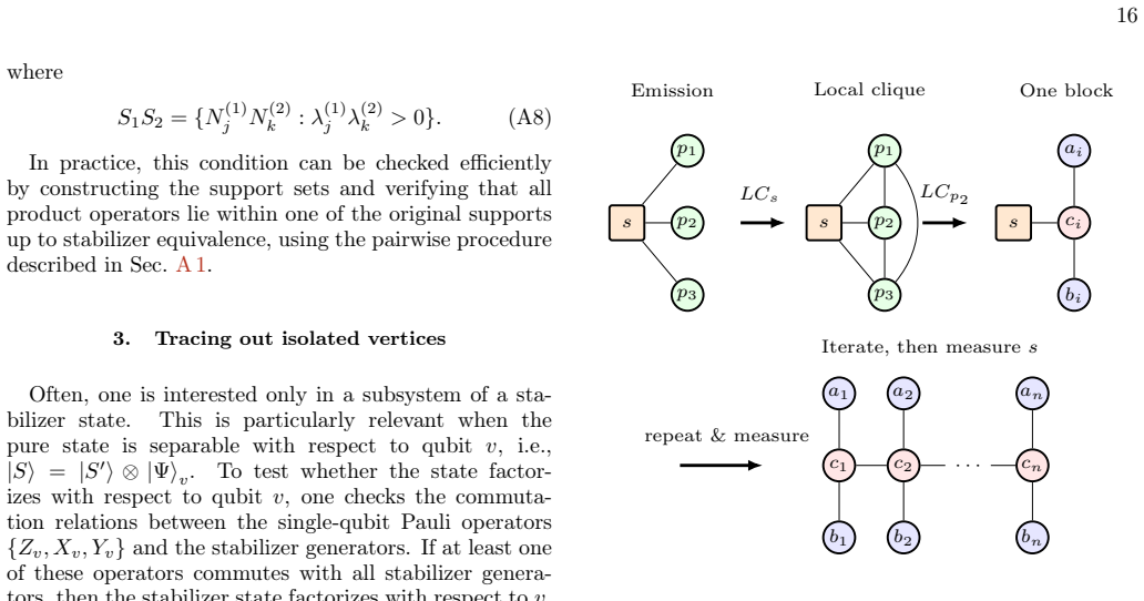
This is particularly relevant when the pure state is separable with respect to qubitv, i.e., |S⟩=|S ′⟩ ⊗ |Ψ⟩ v
Tracing out isolated vertices Often, one is interested only in a subsystem of a sta- bilizer state. This is particularly relevant when the pure state is separable with respect to qubitv, i.e., |S⟩=|S ′⟩ ⊗ |Ψ⟩ v. To test whether the state factor- izes with respect to qubitv, one checks the commuta- tion relations between the single-qubit Pauli operators {Z...
-
[78]
Stochastic mixture of stabilizer states One can consider simulating a stochastic mixture of stabilizer states ρ= X i ci S(i) ED S(i) ,(C1) where S(i) S(i) are different stabilizer states. Consid- ering the noisy simulation of such diagonal states ρ= X i ciE i 1 · · · Ei n S(i) ED S(i) ,(C2) we differentiate again between Clifford update rules, and Pauli-m...
-
[79]
Specifically, one can consider the proba- bilistic application of Clifford unitaries as well as non- deterministic Pauli measurements
Clifford and Pauli measurement noise channels One can also consider the incorporation of noise chan- nels, which are probabilistic applications of operations, which are efficiently treatable by the standard NSF framework. Specifically, one can consider the proba- bilistic application of Clifford unitaries as well as non- deterministic Pauli measurements. ...
discussion (0)
Sign in with ORCID, Apple, or X to comment. Anyone can read and Pith papers without signing in.