Recognition: unknown
Realized Regularized Regressions
Pith reviewed 2026-05-08 08:47 UTC · model grok-4.3
The pith
In high-dimensional continuous-time settings, a group-wise penalized estimator with truncated L1 penalty achieves the oracle property for time-varying coefficient regression and variable selection.
A machine-rendered reading of the paper's core claim, the machinery that carries it, and where it could break.
Core claim
In high-dimensional settings in which the number of candidate covariates diverges, a group-wise penalized estimator with a truncated ℓ1-penalty attains the oracle property, which delivers both consistent model selection and coefficient estimation. The coefficient paths are approximated by spline basis expansions and estimated via least squares from truncated high-frequency increments of Itô semimartingales under infill asymptotics.
What carries the argument
Group-wise penalized least-squares estimator that applies a truncated ℓ1 penalty to the coefficients of spline expansions of the time-varying regression paths, computed from truncated high-frequency increments.
If this is right
- The estimator selects the correct sparse subset of covariates with probability approaching one even as the total number of candidates grows.
- After selection, the coefficient estimator converges at the same rate that would be obtained if the true model were known in advance.
- The same procedure yields a feasible asymptotic distribution for the integrated coefficient estimator in finite-dimensional sub-models.
- Applied to asset-return panels, the method recovers sparse factor structures across large cross-sections of stocks and industry portfolios.
Where Pith is reading between the lines
- The truncation-plus-penalty construction may be portable to other high-frequency regression problems that involve many candidate predictors, such as realized volatility forecasting or macroeconomic nowcasting.
- Replacing splines with other bases (wavelets, Fourier) could capture different smoothness classes while preserving the oracle property under the same truncation scheme.
- The framework suggests a natural way to test whether the sparsity pattern itself changes over time by allowing the penalty to act on groups defined by time intervals.
Load-bearing premise
The response and all candidate covariates must be Itô semimartingales whose jumps can be removed by truncation of high-frequency increments so that the remaining continuous parts support consistent spline-based estimation.
What would settle it
In Monte Carlo data generated from known sparse time-varying coefficients with jumps, the group-wise truncated-L1 estimator either selects the wrong covariates with positive probability or produces coefficient estimates whose integrated squared error fails to match the oracle benchmark.
Figures


read the original abstract
We develop a continuous-time penalized regression framework for the estimation of time-varying coefficients and variable selection when both the response and covariates are It\^o semimartingales with jumps. The coefficient paths are approximated by spline basis expansions and estimated via least squares from truncated high-frequency increments. In a finite-dimensional setting, we establish consistency and derive a feasible asymptotic distribution for the integrated coefficient estimator under infill asymptotics. We then extend the framework to high-dimensional settings in which the number of candidate covariates diverges, and show that a group-wise penalized estimator with a truncated $\ell_1$-penalty attains the oracle property, which delivers both consistent model selection and coefficient estimation. An empirical application to a large panel of more than two hundred high-frequency factors documents sparse factor structure across a large cross-section of stocks and industry portfolios.
Editorial analysis
A structured set of objections, weighed in public.
Referee Report
Summary. The paper develops a continuous-time penalized regression framework for estimating time-varying coefficients and performing variable selection when the response and covariates are Itô semimartingales with jumps. Coefficients are approximated via spline basis expansions and estimated by least squares on truncated high-frequency increments under infill asymptotics. In the finite-dimensional case, consistency and a feasible asymptotic distribution for the integrated coefficient estimator are established. The framework is extended to high-dimensional settings where the number of candidate covariates diverges, with a group-wise estimator using a truncated ℓ1 penalty shown to attain the oracle property (consistent selection and oracle-rate estimation). An empirical application to a panel of over 200 high-frequency factors illustrates sparse factor structure across stocks and portfolios.
Significance. If the oracle property and associated rates hold under the stated conditions, the work would offer a useful extension of penalized regression techniques to continuous-time high-frequency settings with jumps, addressing both time-varying parameters and high-dimensional selection in financial econometrics. The combination of spline approximation, truncation for jumps, and group-wise penalization is technically novel, and the empirical illustration on a large factor panel demonstrates practical relevance.
major comments (2)
- [Abstract and high-dimensional extension] Abstract and high-dimensional extension (presumably §4–5): the claim that the group-wise truncated-ℓ1 estimator attains the oracle property when p diverges rests on the spline-expanded design matrix satisfying uniform restricted-eigenvalue or irrepresentable conditions and on truncation error being negligible relative to the penalty level. However, no explicit growth restrictions are given on p_n relative to the infill frequency or on the spline dimension K_n; if K_n grows at a rate comparable to log p_n, the effective dimension p_n K_n and the summed truncation errors (O_p(Δ^{1/2-ε}) per series) can violate the uniform signal-strength condition required for selection consistency.
- [Finite-dimensional consistency result] Finite-dimensional consistency result (presumably Theorem in §3): while consistency of the integrated coefficient estimator is asserted under infill asymptotics, the feasible asymptotic distribution relies on the truncation threshold being fixed or slowly varying; when extending to the diverging-p case, it is unclear whether the same threshold remains valid or must be adapted to the growing number of series, which is load-bearing for the oracle-rate claim.
minor comments (2)
- [Abstract] The abstract would be clearer if it briefly stated the main growth conditions on p_n and K_n that are required for the oracle property.
- [Model section] Notation for the truncated increments and the group-wise penalty could be introduced earlier with an explicit definition of the truncation threshold.
Simulated Author's Rebuttal
We thank the referee for the constructive and detailed comments on our manuscript. We address each major comment point by point below, clarifying the technical conditions and indicating where revisions will be made to improve rigor and readability.
read point-by-point responses
-
Referee: [Abstract and high-dimensional extension] Abstract and high-dimensional extension (presumably §4–5): the claim that the group-wise truncated-ℓ1 estimator attains the oracle property when p diverges rests on the spline-expanded design matrix satisfying uniform restricted-eigenvalue or irrepresentable conditions and on truncation error being negligible relative to the penalty level. However, no explicit growth restrictions are given on p_n relative to the infill frequency or on the spline dimension K_n; if K_n grows at a rate comparable to log p_n, the effective dimension p_n K_n and the summed truncation errors (O_p(Δ^{1/2-ε}) per series) can violate the uniform signal-strength condition required for selection consistency.
Authors: We agree that explicit growth restrictions are required for the uniform restricted-eigenvalue condition and to keep summed truncation errors negligible relative to the penalty. The original manuscript controls these implicitly via the infill asymptotics and the choice of penalty level λ_n, but we acknowledge the referee's point that this should be stated explicitly. In the revision we will add precise conditions (e.g., K_n = o((log p_n)^{-1}) and p_n = o(n^{1/2-δ}) for δ>0) to the statement of the high-dimensional theorem and the surrounding discussion in Section 4, ensuring the effective dimension p_n K_n and truncation bias remain compatible with selection consistency. revision: yes
-
Referee: [Finite-dimensional consistency result] Finite-dimensional consistency result (presumably Theorem in §3): while consistency of the integrated coefficient estimator is asserted under infill asymptotics, the feasible asymptotic distribution relies on the truncation threshold being fixed or slowly varying; when extending to the diverging-p case, it is unclear whether the same threshold remains valid or must be adapted to the growing number of series, which is load-bearing for the oracle-rate claim.
Authors: The truncation threshold is chosen solely as a function of the sampling interval Δ_n to control the probability of jump contamination uniformly across series; it does not depend on dimension p_n. Under our maintained uniform bounds on the semimartingale characteristics, the same fixed or slowly varying threshold continues to deliver the required error control when p_n diverges polynomially in n. We will insert a short clarifying remark after the finite-dimensional theorem and before the high-dimensional extension to make this uniformity explicit and thereby support the oracle-rate claim. revision: yes
Circularity Check
No circularity: claims rest on standard infill asymptotics and group-lasso oracle theory
full rationale
The derivation proceeds from truncated high-frequency increments of Itô semimartingales, spline expansions of coefficient paths, and a group-wise truncated-ℓ1 penalized least-squares estimator. Consistency and the oracle property are obtained under infill asymptotics with diverging p_n by invoking uniform restricted-eigenvalue conditions on the realized design matrix and standard selection-consistency arguments for group lasso. These steps rely on external high-frequency and high-dimensional estimation theory rather than any self-definition, fitted-input-as-prediction, or load-bearing self-citation chain. No equation reduces to its own input by construction.
Axiom & Free-Parameter Ledger
free parameters (2)
- penalty parameter
- spline basis dimension
axioms (2)
- domain assumption Response and covariates are Itô semimartingales with jumps
- domain assumption Infill asymptotics as mesh of partitions goes to zero
Reference graph
Works this paper leans on
-
[1]
A ¨ ıt-Sahalia, Y., Fan, J., Xue, L., and Zhu, X. (2025a). How a nd when are high-frequency stock returns predictable? Management Science , forthcoming. A ¨ ıt-Sahalia, Y., Jacod, J., and Xiu, D. (2025b). Continuou s-time Fama-MacBeth regressions. Review of Financial Studies , 38(12):3542–3579. A ¨ ıt-Sahalia, Y., Kalnina, I., and Xiu, D. (2020). High-fre...
2020
-
[2]
We have Assumptions 1 and 2 withτ1 → ∞
4.9, Jacod and Protter , 2012), we impose the following stronger assumption than Assumpt ions 1 and 2 without loss of generality: Assumption A.1. We have Assumptions 1 and 2 withτ1 → ∞ . Moreover, the processes β ,β J ,b, ˜b, b′, bβ , σ , ˜σ , σ ′, σ β , c, and the functions δ, ˜δ, δ′, δβ are bounded. Throughout the remainder of Appendix A, references to ...
2012
-
[3]
(iv) (Lemma A.1, Huang et al. , 2004). Let gt = ∑Kn k=1B(k) t γ(k) with γ(k) = (γ(k) 1 ,...,γ (k) p )⊤ ∈ Rp and γ = ((γ(1))⊤,..., (γ(Kn))⊤ )⊤ ∈ RpKn. Then it holds that for any γ ∈ RpKn, ∥g∥2 L2 ≍ p∑ j=1 ∥gj∥2 L2 ≍ ∥γ ∥2 Kn . (A.6) A.2 Proof of Lemma 1 Under Assumption 1 (iii), c is bounded and nonsingular, i.e., there exist constants 0 <κ ≤ κ< ∞ such tha...
2004
-
[4]
Kn∑ k=1 V 2 β j (supp(B(k))) ∫ T 0 /BD {B(k) t >0}dt ≤ (d + 1)|supp(B(k))| Kn∑ k=1 V 2 β j (supp(B(k))) ≤ (d + 1)2Hn Kn∑ k=1 V 2 β j (supp(B(k))). (A.25) 37 Since supp(B(k)) covers at most d + 1 knot intervals and each knot interval belongs to the suppo rts of at most d + 1 B-splines, Kn∑ k=1 V 2 β j (supp(B(k))) ≤ (d + 1)2 Nn+1∑ j=1 V 2 β j ([vj− 1,v j])...
2003
-
[5]
(2004), it holds that sup g∈ Gn ⏐ ⏐ ⏐ ⏐ v⊤ R⊤ Rv v⊤ ˜R⊤ ˜Rv − 1 ⏐ ⏐ ⏐ ⏐ =op(1), (A.31) if ∆ nKn logKn →
By Lemma A.2 in Huang et al. (2004), it holds that sup g∈ Gn ⏐ ⏐ ⏐ ⏐ v⊤ R⊤ Rv v⊤ ˜R⊤ ˜Rv − 1 ⏐ ⏐ ⏐ ⏐ =op(1), (A.31) if ∆ nKn logKn →
2004
-
[6]
Remark A.1 (Predictability)
over the i-th interval is Yi = ∫ i∆ n (i− 1)∆ n β ⊤ s−dXc s + ∑ (i− 1)∆ n≤ s≤ i∆ n (β J s− )⊤ ∆ Xs + ∆ n iZ /BD {|∆ n i Y |≤ un} = ( ∫ i∆ n (i− 1)∆ n ˜β ⊤ s dXc s ) /BD {|∆ n i Y |≤ un} ˜Yi + ( ∫ i∆ n (i− 1)∆ n e⊤ sdXc s ) /BD {|∆ n i Y |≤ un} Ui + ∑ (i− 1)∆ n≤ s≤ i∆ n (β J s− )⊤ ∆ Xs /BD {|∆ n i Y |≤ un} Ji + ∆ n iZ /...
2013
-
[7]
Lemma A.1 is a result from the properties of B-spline basis functions and will be used to derive probabilistic bounds for the compo nents listed above
We start with two lemmas. Lemma A.1 is a result from the properties of B-spline basis functions and will be used to derive probabilistic bounds for the compo nents listed above. Lemma A.2 provides some results regarding the truncation technique o f Mancini (2009), and will be used repeatedly in subsequent proofs. Lemma A.1. For any vector r ∈ Rn, ∥B(R⊤ R)...
2009
-
[8]
44 Finally, by Eqs. ( A.60), ( A.65) and ( A.68), E [ ∥∆ n iX − ∆ n iX c∥2 /BD {∥∆ n i X∥≤ un} ] =O(∆ nu2− r n ), (A.69) and thus, by Markov’s inequality, ∥∆ n iX − ∆ n iX c∥2 /BD {∥∆ n i X∥≤ un} =Op(∆ nu2− r n ). (A.70) This completes the proof of Lemma A.2 (ii). Next, we verify that A1, A2, A3 and A4 in Eq. ( A.36) are all op(1): (i) A1 = op(1). We cons...
1973
-
[9]
(A.94) by Eqs
( ∫ i∆ n (i− 1)∆ n ∫ {∥δ∥≤ un/ 2} ∥δ(s,x )∥µ (ds,dx ) )] + 2 un E [ N n i (2un) ( ∫ i∆ n (i− 1)∆ n ∫ {∥δ∥≤ un/ 2} ∥δ(s,x )∥µ (ds,dx ) )] ≤ K un (∆ nu− r n )2(∆ nu1− r n ) + K ′ un (∆ nu− r n )(∆ nu1− r n ) ≤ K ′∆ 2 nu− 2r n . (A.94) by Eqs. ( A.38) and ( A.40), and the fact that {∥δ(s,x )∥> 2un} and {∥δ(s,x )∥ ≤ un/ 2} are disjoint. Combining Eqs. ( A.92)...
2012
-
[10]
( A.104), we consider a further decomposition by Eq
For the fixed linear combination in Eq. ( A.104), we consider a further decomposition by Eq. ( A.35): Hn = 1√ ∆ n a⊤ ( n∑ i=1 B(i− 1)∆ n ∆ n ) (R⊤ R)− 1R⊤ ( ˜Y − Rγ ) H1,n + 1√ ∆ n a⊤ ( n∑ i=1 B(i− 1)∆ n ∆ n ) (R⊤ R)− 1R⊤ U H2,n + 1√ ∆ n a⊤ ( n∑ i=1 B(i− 1)∆ n ∆ n ) (R⊤ R)− 1R⊤ J H3,n + 1√ ∆ n a⊤ ( n∑ i=1 B(i− 1)∆ n∆ n ) (R⊤ R)− 1R⊤ Z,...
2012
-
[11]
We define a permutation matrix P that reorders elements in R (group the p components associated with each spline basis index)
Firstly, the local support of B-splines imply that ( n∑ i=1 B(i− 1)∆ n ∆ n ) ⊤ a ∞ ≤ K∥a∥∞ max 1≤ k≤ Kn n∑ i=1 B(k) (i− 1)∆ n ∆ n ≤ K∥a∥∞ sup t∈ [0,T ] B(k) t ( ⌈ |supp(B(k))| ∆ n ⌉ + 1 ) ∆ n ≤ K ′ Kn , (A.118) where |supp(B(k))| ≍ K − 1 n ; see Appendix A.1 (iii). We define a permutation matrix P that reorders elements in R (group ...
1984
-
[12]
( A.207) and ( A.208)
68 Term (5): By Markov’s inequality, unP ( |˜Ji|>u n ) ≤ un E[|˜Ji|] un ≤ E[|˜Ji|] ≤ K∆ nu1− r n , (A.221) which can be calculated following the same steps as in Eqs. ( A.207) and ( A.208). Term (6): By H¨ older’s inequality, for someq ≥ 2, E [ |∆ n iY (1)| /BD {|˜Ji|>un} ] ≤ ( E[|∆ n iY (1)|q] ) 1/q ( P ( |˜Ji|>u n )) 1− 1/q ≤ K √ ∆ n(∆ nu− r n )1− 1/q =...
2012
-
[13]
Inactive blocks
Hence the active-block KKT conditions hold. Inactive blocks. Forq + 1 ≤ j ≤ p, ˆγ◦ j ≡ 0 by construction. Under the condition λ n τn / ( √ ∆ n logpKn Kn +un logpKn +u1− r/ 2 n ) → ∞ , (A.260) it suffices to show max q+1≤ j≤ p √ (cj (ˆγ ◦))⊤ Wjcj(ˆγ ◦) = Op ( √ ∆ n logpKn Kn +un logpKn +u1− r/ 2 n ) , (A.261) which implies Eq. ( A.255). By Eq. ( A.257), we h...
2008
-
[14]
(A.297) Proof of Lemma A.5. Define the residualized block as ˜R∗ j = MA◦ R∗ j ∈ Rn× Kn, the projection matrix H∗ j = ˜R∗ j (( ˜R∗ j )⊤ ˜R∗ j )− 1( ˜R∗ j )⊤ ∈ Rn× n onto span( ˜R∗ j ), and the corresponding residualizer 80 M∗ j = In − H∗ j . By the Frisch-Waugh-Lovell theorem (Theorem 2.1, Davidson and MacKinnon , 2004), the OLS residual sums of squares fro...
2004
-
[15]
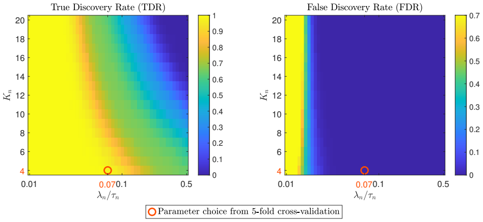
The number of B-spline basis functions Kn and the effective penalty level λ n/τ n are selected via 5-fold cross-validation
The cutoff level i n the TLP function is τn = α τ √ MedR VT for each simulated path of Y . The number of B-spline basis functions Kn and the effective penalty level λ n/τ n are selected via 5-fold cross-validation. AKX stands for the estimator of A ¨ ıt-Sahalia et al.(2020). For both the spline-based and AKX estimators, the truncat ion thresholds for the in...
2020
-
[16]
The cutoff level in the TLP function is τn = α τ √ MedR VT for each simulated path of Y
The modified simu lation design allows dependence among the redundant factor s and also correlations between relevant and redundant factors. The cutoff level in the TLP function is τn = α τ √ MedR VT for each simulated path of Y . The number of B-spline basis functions Kn and the effective penalty level λ n/τ n are selected via 5-fold cross-validation. AKX s...
2020
-
[17]
F actor selection
JNJ Johnson & Johnson 35 Health Care 2834 Pharmaceutical Pro ducts (13) JPM JPMorgan Chase & Co 40 Financials 6020 Banking (44) LLY Eli Lilly & Co 35 Health Care 2834 Pharmaceutical Product s (13) LMT Lockheed Martin Corp 20 Industrials 3760 Defense (26) LOW Lowe’s Cos Inc 25 Consumer Discretionary 5211 Retail (42 ) MA Mastercard Inc 40 Financials 7389 Bu...
2080
-
[18]
Sector cl assifications are based on the GICS sector code from WRDS Comp ustat
UPS UPS 20 Industrials 4210 Transportation (40) V Visa Inc 40 Financials 6099 Banking (44) VZ Verizon Communications Inc 50 Communication Services 48 12 Communication (32) WBA W algreens Boots Alliance Inc 30 Consumer Staples 5912 Re tail (42) WFC W ells Fargo & Co 40 Financials 6020 Banking (44) WMT W almart Inc 30 Consumer Staples 5331 Retail (42) XOM E...
2016
discussion (0)
Sign in with ORCID, Apple, or X to comment. Anyone can read and Pith papers without signing in.