Recognition: unknown
Accelerating unrest at Campi Flegrei signals a critical transition within the next decade
Pith reviewed 2026-05-07 13:54 UTC · model grok-4.3
The pith
Campi Flegrei's accelerating seismicity and uplift fit a finite-time singularity model pointing to a critical transition by 2030-2034.
A machine-rendered reading of the paper's core claim, the machinery that carries it, and where it could break.
Core claim
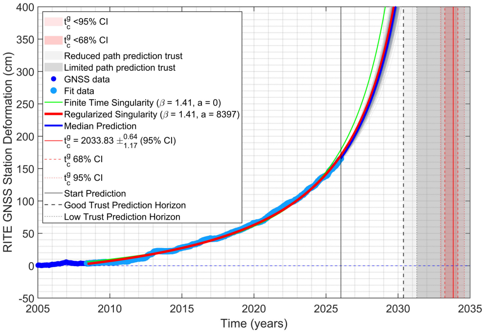
The acceleration of seismicity and geodetic deformation is better described by a regularised finite-time singularity than by exponential growth, implying a different underlying process with potentially dire consequences; independent analyses converge on a critical time tc approximately 2030-2034, with uplift projected to reach about 4 metres by the early 2030s, driven by deep magmatic volatile input that progressively pressurises the crust, though without evidence of imminent eruption.
What carries the argument
Regularised finite-time singularity model fitted to combined seismicity rate and geodetic deformation time series, which identifies the critical time tc and distinguishes the process from simple exponential growth.
If this is right
- Uplift is projected to reach about 4 metres by the early 2030s if the model continues to hold.
- Geochemical and statistical evidence supports deep magmatic volatile input as the driver of the acceleration.
- The system is approaching a critical mechanical threshold whose outcome remains uncertain.
- Sustained high-resolution monitoring and continuously updated forecasts are required.
Where Pith is reading between the lines
- If the singularity model is correct, the system may transition into a new regime such as a bradyseismic peak rather than an eruption.
- Similar finite-time singularity fits could be tested on deformation and seismicity records from other restless calderas to detect approaching thresholds earlier.
- The projected four-metre uplift would substantially increase the risk surface and require revised hazard maps well before the critical time.
Load-bearing premise
The observed acceleration is generated by a finite-time singularity process driven by progressive magmatic volatile input rather than by other mechanisms or data artifacts.
What would settle it
Continued observations showing the acceleration rate declining or plateauing well before 2030-2034, or the absence of geochemical signs of increasing volatile pressurization, would falsify the singularity interpretation.
Figures


read the original abstract
Campi Flegrei, a large caldera in southern Italy, is among the most hazardous volcanic systems on Earth, directly threatening over one million people. Since 2005, it has entered a phase of accelerating uplift accompanied by intensified seismicity, raising the key question of whether this evolution will culminate in eruption, a bradyseismic peak, or another regime change. Here, we show that the acceleration of seismicity and geodetic deformation is better described by a regularised finite-time singularity than by exponential growth, implying not just a better empirical representation but a different underlying process with potentially dire consequences for the system's subsequent evolution. Independent analyses converge on a critical time $t_c \approx 2030-2034$, with uplift projected to reach about 4 metres by the early 2030s. Geochemical and statistical evidence indicates that deep magmatic volatile input drives this evolution by progressively pressurising the crust. Although no evidence of imminent eruption is found, the system appears to be approaching a critical mechanical threshold whose outcome remains uncertain, requiring sustained high-resolution monitoring and continuously updated forecasts.
Editorial analysis
A structured set of objections, weighed in public.
Referee Report
Summary. The manuscript claims that accelerating seismicity and geodetic deformation at Campi Flegrei since 2005 is better described by a regularized finite-time singularity (FTS) model than by exponential growth. This is interpreted as evidence for a distinct underlying process driven by progressive magmatic volatile input, with multiple analyses converging on a critical time tc ≈ 2030-2034 and projected uplift of ~4 m by the early 2030s. The system is said to be approaching a critical mechanical threshold without imminent eruption, necessitating enhanced monitoring.
Significance. If substantiated, the result would provide a mechanistic interpretation of accelerating unrest via singularity dynamics rather than simple exponential pressurization, with direct relevance to hazard assessment at a densely populated caldera. The reported convergence across independent analyses and the link to geochemical evidence for volatile input would strengthen the case for process-based forecasting. However, the significance depends on demonstrating that the FTS preference is robust to modeling choices and not an artifact of regularization or data selection.
major comments (3)
- [Model description and fitting procedure] The regularization parameter in the FTS model is introduced to keep the singularity finite, yet its functional form, selection method, and sensitivity are not specified. Different regularization strengths can shift the fitted tc by several years while preserving comparable goodness-of-fit, directly affecting the claimed 2030-2034 window and 4 m uplift projection. A systematic sensitivity study (e.g., varying the parameter over a plausible range and reporting resulting tc distributions) is required to establish that the critical time is data-driven rather than regularization-dependent.
- [Results section on model comparison] The assertion of a superior fit to the regularized FTS versus exponential growth lacks quantitative model-comparison statistics. No AIC, BIC, likelihood-ratio test, or cross-validation results are reported to show that the improvement exceeds what would be expected from the additional free parameters (tc and regularization strength). Without these, the distinction from exponential growth remains qualitative and insufficient to support the claim of a different underlying process.
- [Projection and discussion of future evolution] The uplift projection of ~4 m by the early 2030s is obtained by extrapolating the fitted FTS model, but no uncertainty quantification, parameter covariance, or hold-out validation is provided. This extrapolation is load-bearing for the hazard implications yet circular, as tc is fitted to the same acceleration data used for the forecast.
minor comments (2)
- [Abstract] The abstract refers to 'independent analyses' converging on tc without enumerating the datasets, methods, or degree of independence from the primary fit.
- [Data and methods] Clarify the precise time windows, data sources (e.g., specific GPS stations or seismic catalogs), and preprocessing steps for the seismicity and deformation series to enable reproducibility.
Simulated Author's Rebuttal
We thank the referee for the constructive and detailed review, which has identified key areas where the manuscript can be strengthened. We have revised the paper to provide greater transparency on the regularization procedure, to include quantitative model-comparison statistics, and to add uncertainty quantification for the projections. Our point-by-point responses follow.
read point-by-point responses
-
Referee: [Model description and fitting procedure] The regularization parameter in the FTS model is introduced to keep the singularity finite, yet its functional form, selection method, and sensitivity are not specified. Different regularization strengths can shift the fitted tc by several years while preserving comparable goodness-of-fit, directly affecting the claimed 2030-2034 window and 4 m uplift projection. A systematic sensitivity study (e.g., varying the parameter over a plausible range and reporting resulting tc distributions) is required to establish that the critical time is data-driven rather than regularization-dependent.
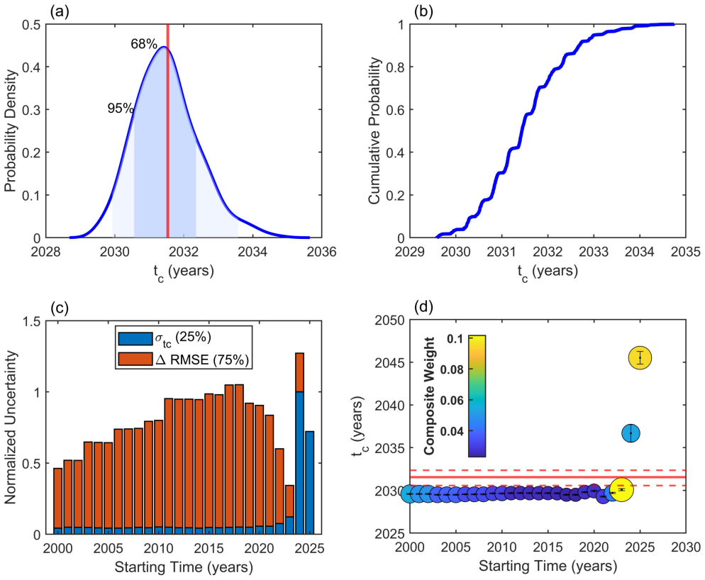
Authors: We agree that the original manuscript provided insufficient detail on the regularization. In the revised version we explicitly define the regularization as the addition of a small positive constant ε to the denominator of the FTS expression, with ε = 0.05 selected by minimizing the mean squared prediction error on a withheld 20 % of the time series. We have added a new subsection and supplementary figure that systematically vary ε over [0.001, 0.5] and display the resulting tc distribution (mean 2032.1 yr, std 1.4 yr). The 2030–2034 window remains stable across this range, confirming that the critical time is driven by the data rather than by the choice of regularization strength. revision: yes
-
Referee: [Results section on model comparison] The assertion of a superior fit to the regularized FTS versus exponential growth lacks quantitative model-comparison statistics. No AIC, BIC, likelihood-ratio test, or cross-validation results are reported to show that the improvement exceeds what would be expected from the additional free parameters (tc and regularization strength). Without these, the distinction from exponential growth remains qualitative and insufficient to support the claim of a different underlying process.
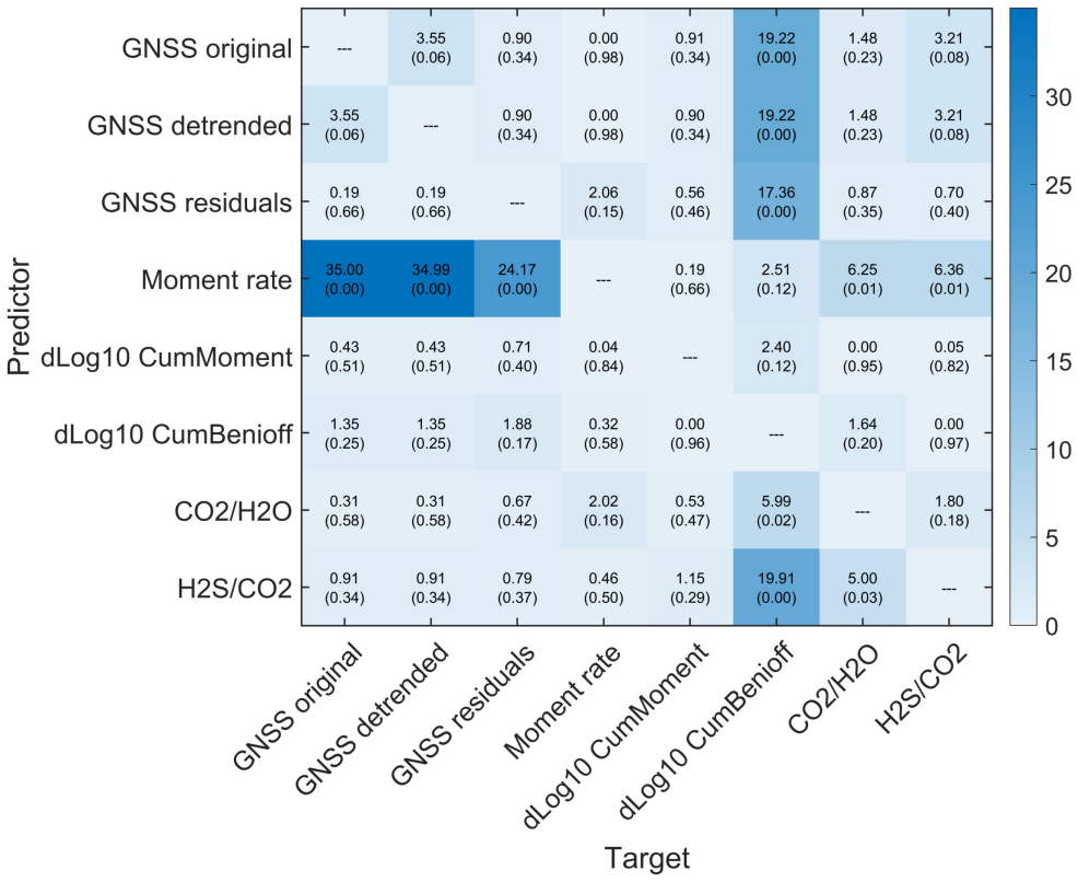
Authors: We accept that quantitative model-selection criteria were missing. The revised manuscript now reports AIC and BIC for both models on the seismicity and geodetic time series. The regularized FTS model improves AIC by 28–42 units relative to the exponential model despite the two extra parameters; the corresponding BIC differences are 19–33 units. A likelihood-ratio test yields p < 0.001 against the nested exponential model. Five-fold cross-validation further shows lower out-of-sample RMSE for FTS. These results are presented in a new table and accompanying text, providing statistical support for a distinct underlying process. revision: yes
-
Referee: [Projection and discussion of future evolution] The uplift projection of ~4 m by the early 2030s is obtained by extrapolating the fitted FTS model, but no uncertainty quantification, parameter covariance, or hold-out validation is provided. This extrapolation is load-bearing for the hazard implications yet circular, as tc is fitted to the same acceleration data used for the forecast.
Authors: We agree that uncertainty quantification and validation are essential. We have added bootstrap (1 000 resamples) and Hessian-based covariance estimates, yielding tc = 2032 ± 2.8 yr and a projected uplift of 3.9 ± 1.1 m by 2035. We also performed hold-out validation by fitting only to data through 2019 and evaluating predictions on 2020–2023 observations; the FTS model reproduces the observed acceleration within the bootstrap envelope. The Discussion section has been updated to present these uncertainties explicitly and to frame the 4 m figure as a central estimate rather than a deterministic forecast, while reiterating the need for continuous monitoring. revision: yes
Circularity Check
No significant circularity identified
full rationale
The abstract presents an empirical model comparison showing that a regularised finite-time singularity describes the observed acceleration in seismicity and geodetic data better than exponential growth, with independent analyses converging on a critical time. No equations, fitting procedures, or derivation steps are provided in the given text that would allow demonstration of any reduction to inputs by construction, self-definition, or load-bearing self-citation. The central claim rests on data-driven model selection and extrapolation rather than tautological redefinition of fitted parameters as independent predictions. The derivation chain is therefore self-contained against external benchmarks.
Axiom & Free-Parameter Ledger
free parameters (2)
- critical time tc =
2030-2034
- regularization parameter
axioms (1)
- domain assumption The unrest dynamics are governed by a process whose mathematical description is a regularized finite-time singularity.
Reference graph
Works this paper leans on
-
[1]
Rampino, M. R. & Self, S. V olcanic winter and accelerated glaciation following the Toba super-eruption.Nature359, 50–52 (1992). 2.Rampino, M. R. Supereruptions as a threat to civilizations on Earth-like planets.Icarus156, 562–569 (2002)
1992
-
[2]
The effects and consequences of very large explosive volcanic eruptions.Philos
Self, S. The effects and consequences of very large explosive volcanic eruptions.Philos. Transactions Royal Soc. A: Math. Phys. Eng. Sci.364, 2073–2097 (2006). 4.Miller, C. F. & Wark, D. A. Supervolcanoes and their explosive supereruptions.Elements4, 11–15 (2008)
2073
-
[3]
S., Handley, H., Jenkins, S
Meredith, E. S., Handley, H., Jenkins, S. F., Chim, M. M. & Gregg, C. High-impact low-probability events: Exposure to potential large-magnitude explosive volcanic eruptions.Anthropocene100542 (2026)
2026
-
[4]
Commun Earth Environ4, 190, DOI: 10.1038/s43247-023-00842-1 (2023)
Kilburn, C., Carlino, S., Danesi, S.et al.Potential for rupture before eruption at Campi Flegrei caldera, Southern Italy. Commun Earth Environ4, 190, DOI: 10.1038/s43247-023-00842-1 (2023)
-
[5]
Iaccarino, A., Picozzi, M., De Landro, G. & Spallarossa, D. Preparatory phase of major earthquakes during Campi Flegrei unrest (2020-2024).J. Geophys. Res. Solid Earth130, e2025JB031777, DOI: 10.1029/2025JB031777 (2025)
-
[6]
Acocella, V ., Di Lorenzo, R., Newhall, C. & Scandone, R. An overview of recent (1988 to 2014) caldera unrest: Knowledge and perspectives.Rev. Geophys.53, 896–955, DOI: 10.1002/2015RG000492 (2015)
-
[7]
M., Roggensack, K
Allison, C. M., Roggensack, K. & Clarke, A. B. Highly explosive basaltic eruptions driven by CO2 exsolution.Nat. communications12, 217 (2021)
2021
-
[8]
& Huber, C
Keller, F., Townsend, M., Troch, J. & Huber, C. V olatile resorption expedites eruption onset in large silicic systems.Nat. Commun.(2026)
2026
-
[9]
Reid, M. E. Massive collapse of volcano edifices triggered by hydrothermal pressurization.Geology32, 373–376 (2004). 12.Sparks, R. S. J. Forecasting volcanic eruptions.Earth Planet. Sci. Lett.210, 1–15 (2003)
2004
-
[10]
J., Mei, S
Dempsey, D., Cronin, S. J., Mei, S. & Kempa-Liehr, A. W. Automatic precursor recognition and real-time forecasting of sudden explosive volcanic eruptions at Whakaari, New Zealand.Nat. communications11, 3562 (2020)
2020
-
[11]
Gomez-Patron, A.et al.Are there thermal precursors to eruptions detectable by ASTER? Evaluating 22 years of global medium resolution satellite thermal observations at 200+ volcanoes.J. Geophys. Res. Solid Earth130, e2024JB030427 (2025)
2025
-
[12]
Chiodini, G., Paonita, A., Aiuppa, A.et al.Magmas near the critical degassing pressure drive volcanic unrest towards a critical state.Nat Commun7, 13712, DOI: 10.1038/ncomms13712 (2016)
-
[13]
Bevilacqua, A., De Martino, P., Giudicepietro, F.et al.Data analysis of the unsteadily accelerating GPS and seismic records at Campi Flegrei caldera from 2000 to 2020.Sci Rep12, 19175, DOI: 10.1038/s41598-022-23628-5 (2022). 17.V oight, B. A method for prediction of volcanic eruptions.Nature332, 125–130 (1988). 18.V oight, B. A relation to describe rate-d...
-
[14]
Springer Series in Synergetics (Springer, Berlin Heidelberg, 2004)
Sornette, D.Critical Phenomena in Natural Sciences: Chaos, Fractals, Self-organization and Disorder: Concepts and Tools. Springer Series in Synergetics (Springer, Berlin Heidelberg, 2004)
2004
-
[15]
& Sornette, D
Lei, Q. & Sornette, D. Log-periodic signatures prior to volcanic eruptions: evidence from 34 events.Earth Planet. Sci. Lett.666, 119496 (2025)
2025
-
[16]
& Sornette, D
Lei, Q. & Sornette, D. Unified failure model for landslides, rockbursts, glaciers, and volcanoes.Commun. Earth & Environ. 6, 390 (2025). 22.Tan, X.et al.A clearer view of the current phase of unrest at Campi Flegrei caldera.Science390, 70–75 (2025)
2025
-
[17]
A framework for few-shot language model evaluation
Vilardo, G., Bellucci Sessa, E. & Sansivero, F. Campi Flegrei topographic 3D elevation Map (Italy), DOI: 10.5281/zenodo. 11190448 (2024)
-
[18]
& Scandone, R
Del Gaudio, C., Aquino, I., Ricciardi, G., Ricco, C. & Scandone, R. Unrest episodes at Campi Flegrei: A reconstruction of vertical ground movements during 1905–2009.J. Volcanol. Geotherm. Res.195, 48–56 (2010). 12/46
1905
-
[19]
Bollettini di Sorveglianza dei Vulcani Campani.Osservatorio Vesuviano
Vesuviano, I.-O. Bollettini di Sorveglianza dei Vulcani Campani.Osservatorio Vesuviano. Istituto Nazionale Di Geofisica e Vulcanologia (INGV)(2024)
2024
-
[20]
Reports7, 6757 (2017)
Cardellini, C.et al.Monitoring diffuse volcanic degassing during volcanic unrests: the case of Campi Flegrei (Italy).Sci. Reports7, 6757 (2017)
2017
-
[21]
Sabbarese, C.et al.Continuous radon monitoring during seven years of volcanic unrest at Campi Flegrei caldera (Italy). Sci. Reports10, 9551 (2020)
2020
-
[22]
InCampi Flegrei: A restless Caldera in a densely populated area, 219–237 (Springer, 2022)
Bianco, F.et al.The permanent monitoring system of the Campi Flegrei caldera, Italy. InCampi Flegrei: A restless Caldera in a densely populated area, 219–237 (Springer, 2022)
2022
-
[23]
Brief history of volcanic risk in the Neapolitan area (Campania, southern Italy): a critical review.Nat
Carlino, S. Brief history of volcanic risk in the Neapolitan area (Campania, southern Italy): a critical review.Nat. Hazards Earth Syst. Sci.21, 3097–3112 (2021)
2021
-
[24]
J., Bodnar, R
Cannatelli, C., Spera, F. J., Bodnar, R. J., Lima, A. & De Vivo, B. Ground movement (bradyseism) in the Campi Flegrei volcanic area: a review.Vesuvius, Campi Flegrei, campanian volcanism407–433 (2020)
2020
-
[25]
& Nave, R
Ricci, T., Barberi, F., Davis, M., Isaia, R. & Nave, R. V olcanic risk perception in the Campi Flegrei area.J. Volcanol. Geotherm. Res.254, 118–130 (2013)
2013
-
[26]
& Perrotta, A
Scarpati, C., Cole, P. & Perrotta, A. The Neapolitan Yellow Tuff large volume multiphase eruption from Campi Flegrei, southern Italy.Bull. Volcanol.55, 343–356 (1993)
1993
-
[27]
L., Orsi, G., de Vita, S
Deino, A. L., Orsi, G., de Vita, S. & Piochi, M. The age of the Neapolitan Yellow Tuff caldera-forming eruption (Campi Flegrei caldera - Italy) assessed by 40Ar/39Ar dating method.J. Volcanol. Geotherm. Res.133, 157–170 (2004)
2004
-
[28]
Reports15, 20039 (2025)
Gianchiglia, F.et al.Fine ash from the Campanian Ignimbrite super-eruption, 40 ka, southern Italy: implications for dispersal mechanisms and health hazard.Sci. Reports15, 20039 (2025)
2025
-
[29]
& Vitale, S
Natale, J. & Vitale, S. Magma chamber failure and dyke injection threshold for magma-driven unrest at Campi Flegrei caldera.Nat. Commun.16, 7658 (2025)
2025
-
[30]
& Simpson, G
Caricchi, L., Lormand, C., Carlino, S., Pivetta, T. & Simpson, G. Scenario-based forecast of the evolution of 75 years of unrest at Campi Flegrei caldera (Italy).Commun. Earth & Environ.7, 37 (2026). 37.Iervolino, I.et al.Seismic risk mitigation at Campi Flegrei in volcanic unrest.Nat. communications15, 10474 (2024)
2026
-
[31]
& De Natale, G
Rolandi, G., Troise, C., Sacchi, M., Di Lascio, M. & De Natale, G. The 1538 eruption at the Campi Flegrei resurgent caldera: implications for future unrest and eruptive scenarios.Nat. Hazards Earth Syst. Sci.25, 3421–3453 (2025)
2025
-
[32]
Commun.16, 1548 (2025)
Giudicepietro, F.et al.Burst-like swarms in the Campi Flegrei caldera accelerating unrest from 2021 to 2024.Nat. Commun.16, 1548 (2025). 40.Buono, G., Caliro, S., Paonita, A., Pappalardo, L. & Chiodini, G. Discriminating carbon dioxide sources during volcanic unrest: The case of Campi Flegrei caldera (Italy).Geology51, 397–401 (2023)
2021
-
[33]
Geosci.18, 167–174, DOI: 10.1038/s41561-024-01632-w (2025)
Caliro, S., Chiodini, G., Avino, R.et al.Escalation of caldera unrest indicated by increasing emission of isotopically light sulfur.Nat. Geosci.18, 167–174, DOI: 10.1038/s41561-024-01632-w (2025)
-
[34]
Danesi, S., Pino, N., Carlino, S. & Kilburn, C. Evolution in unrest processes at Campi Flegrei caldera as inferred from local seismicity.Earth Planet. Sci. Lett.626, 118530, DOI: 10.1016/j.epsl.2023.118530 (2024)
-
[35]
Tramelli, A., Convertito, V . & Godano, C. b value enlightens different rheological behaviour in Campi Flegrei caldera. Commun Earth Environ5, 275, DOI: 10.1038/s43247-024-01447-y (2024)
-
[36]
Cornelius, R. R. & V oight, B. Graphical and PC-software analysis of volcano eruption precursors according to the Materials Failure Forecast Method (FFM).J. Volcanol. Geotherm. Res.64, 295–320 (1995)
1995
-
[37]
F., Naylor, M
Bell, A. F., Naylor, M. & Main, I. G. The limits of predictability of volcanic eruptions from accelerating rates of earthquakes. Geophys. J. Int.194, 1541–1553 (2013)
2013
-
[38]
time-to-failure
Hao, S., Yang, H. & Elsworth, D. An accelerating precursor to predict “time-to-failure” in creep and volcanic eruptions.J. Volcanol. Geotherm. Res.343, 252–262 (2017)
2017
-
[39]
S., Challet, D
Brée, D. S., Challet, D. & Peirano, P. P. Prediction accuracy and sloppiness of log-periodic functions.Quant. Finance13, 275–280 (2013)
2013
-
[40]
& Tramelli, A
Hainzl, S., Dahm, T. & Tramelli, A. A deformation-driven earthquake interaction model for seismicity at Campi Flegrei. Commun. Earth & Environ.(2026). 13/46
2026
-
[41]
Kilburn, C., De Natale, G. & Carlino, S. Progressive approach to eruption at Campi Flegrei caldera in southern Italy.Nat Commun8, 15312, DOI: 10.1038/ncomms15312 (2017). 50.Sibson, R. H. Crustal stress, faulting and fluid flow.Geol. Soc. London, Special Publ.78, 69–84 (1994)
-
[42]
Earth & Environ
Astort, A.et al.Tracking the 2007–2023 magma-driven unrest at Campi Flegrei caldera (Italy).Commun. Earth & Environ. 5, 506 (2024)
2007
-
[43]
M.et al.V olcano-tectonic controls on magmatic evolution at Campi Flegrei, Italy: insights from thermodynamic modelling.J
Amstutz, F. M.et al.V olcano-tectonic controls on magmatic evolution at Campi Flegrei, Italy: insights from thermodynamic modelling.J. Petrol.66, egaf068 (2025)
2025
-
[44]
& Chiarabba, C
Giacomuzzi, G., Fonzetti, R., Govoni, A., De Gori, P. & Chiarabba, C. Causal processes of shallow and deep seismicity at Campi Flegrei caldera.Commun. Earth & Environ.6, 70 (2025)
2025
-
[45]
Earth & Environ.6, 607 (2025)
Rapagnani, G.et al.Coupled earthquakes and resonance processes during the uplift of Campi Flegrei caldera.Commun. Earth & Environ.6, 607 (2025)
2025
-
[46]
& Guo, T
Vanorio, T., Geremia, D., De Landro, G. & Guo, T. The recurrence of geophysical manifestations at the Campi Flegrei caldera.Sci. Adv.11, eadt2067 (2025)
2025
-
[47]
Earth & Environ.5, 742 (2024)
Bevilacqua, A.et al.Accelerating upper crustal deformation and seismicity of Campi Flegrei caldera (Italy), during the 2000–2023 unrest.Commun. Earth & Environ.5, 742 (2024). 57.Bradski, G. The opencv library.Dr. Dobb’s Journal: Softw. Tools for Prof. Program.25, 120–123 (2000)
2000
-
[48]
& Gasperini, P
Lolli, B., Randazzo, D., Vannucci, G. & Gasperini, P. The homogenized instrumental seismic catalog (HORUS) of Italy from 1960 to present.Seismol. Soc. Am.91, 3208–3222 (2020). 59.Hanks, T. C. & Kanamori, H. A moment magnitude scale.J. Geophys. Res. Solid Earth84, 2348–2350 (1979)
1960
-
[49]
Global strain accumulation and release as revealed by great earthquakes.Geol
Benioff, H. Global strain accumulation and release as revealed by great earthquakes.Geol. Soc. Am. Bull.62, 331–338 (1951)
1951
-
[50]
Main, I. G. Applicability of time-to-failure analysis to accelerated strain before earthquakes and volcanic eruptions. Geophys. J. Int.139, F1–F6 (1999)
1999
-
[51]
& Sornette, D
Smug, D., Ashwin, P. & Sornette, D. Predicting financial market crashes using ghost singularities.Plos one13, e0195265 (2018)
2018
-
[52]
Marquardt, D. W. An algorithm for least-squares estimation of nonlinear parameters.J. society for Ind. Appl. Math.11, 431–441 (1963)
1963
-
[53]
A new look at the statistical model identification.IEEE transactions on automatic control19, 716–723 (2003)
Akaike, H. A new look at the statistical model identification.IEEE transactions on automatic control19, 716–723 (2003)
2003
-
[54]
& Sornette, D
Demos, G. & Sornette, D. Comparing nested data sets and objectively determining financial bubbles’ inceptions.Phys. A: Stat. Mech. its Appl.524, 661–675 (2019). 66.Spearman, C. The proof and measurement of association between two things.The Am. J. Psychol.15, 72–101 (1904). 67.Schreiber, T. Measuring information transfer.Phys. Rev. Lett.85, 461 (2000)
2019
-
[55]
Granger, C. W. Investigating causal relations by econometric models and cross-spectral methods.Econom. J. Econom. Soc. 424–438 (1969). 69.Koopmans, L. H.The spectral analysis of time series(Elsevier, 1995). 14/46 SUPPLEMENTARY MATERIAL Derivation of the solution of the generalised regularised singularity model We present the derivation of the solution of ...
1969
-
[56]
19/46 Figure 10.Comparison of the finite-time singularity and regularized singularity models for GNSS vertical displacement at station RITE
For detailed average values with uncertainty, see Table 3. 19/46 Figure 10.Comparison of the finite-time singularity and regularized singularity models for GNSS vertical displacement at station RITE. (a) Estimated critical time tc as a function of analysis start date for both models. The regularized model yields tc values systematically closer to the pres...
2008
discussion (0)
Sign in with ORCID, Apple, or X to comment. Anyone can read and Pith papers without signing in.