Recognition: unknown
On the use of satellite information to estimate agricultural carbon footprint in a small area framework
Pith reviewed 2026-05-07 14:12 UTC · model grok-4.3
The pith
Satellite ammonia emission data improves accuracy and stability of small-area agricultural carbon footprint estimates.
A machine-rendered reading of the paper's core claim, the machinery that carries it, and where it could break.
Core claim
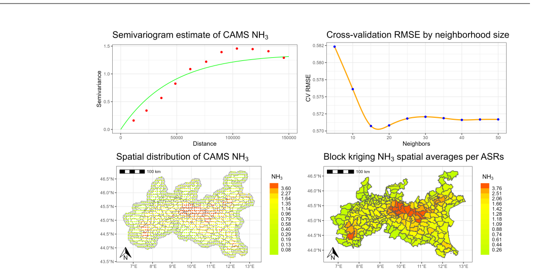
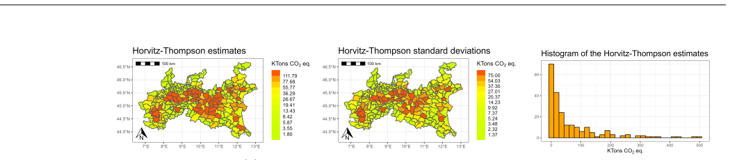
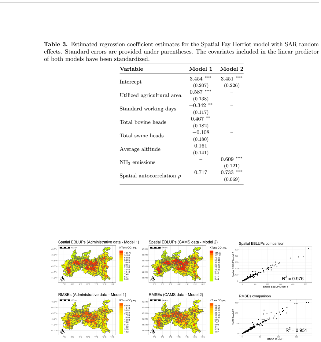
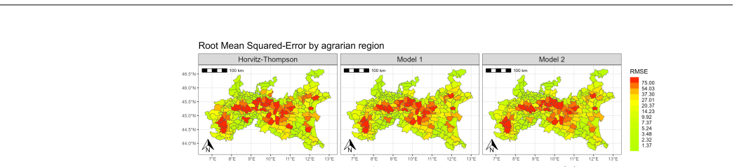
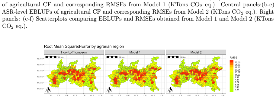
The authors establish that incorporating satellite-derived ammonia emission data into a small-area estimation model substantially improves the accuracy and stability of carbon footprint estimates for agriculturally homogeneous municipalities while reducing dependence on large auxiliary datasets; the spatial misalignment between gridded satellite data and administrative units is handled through a geostatistical upscaling procedure whose uncertainty is propagated via parametric bootstrap.
What carries the argument
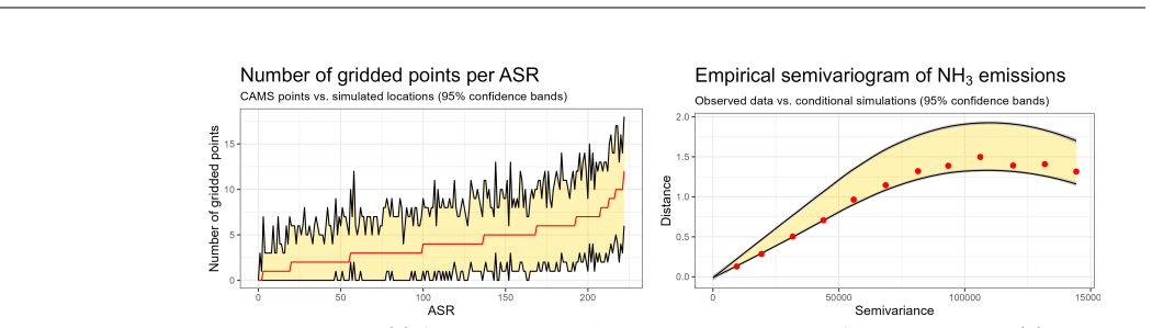
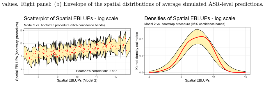
Geostatistical upscaling procedure that aligns gridded satellite ammonia emission data to agrarian subregion boundaries, combined with parametric bootstrap to propagate uncertainty from covariate construction.
If this is right
- Subregional carbon footprint estimates become more precise and spatially coherent without requiring extensive heterogeneous auxiliary surveys.
- Policy-relevant environmental indicators can be produced at finer scales in data-constrained agricultural zones.
- The framework reduces overall reliance on traditional large-scale datasets for similar environmental statistics.
- Uncertainty from auxiliary data construction is explicitly accounted for in the published estimates.
Where Pith is reading between the lines
- The same satellite-augmented approach could extend to estimating other livestock-related emissions or environmental burdens in comparable intensive farming regions.
- Official statistical agencies might adopt Earth-observation covariates to lower costs of maintaining fine-scale sustainability indicators.
- If the proxy relationship holds, the method offers a scalable template for integrating remote-sensing data into model-based small-area statistics beyond agriculture.
Load-bearing premise
Satellite ammonia emission data acts as an accurate, unbiased proxy for agricultural carbon emissions and the upscaling procedure aligns gridded data to boundaries without material bias or unaccounted error.
What would settle it
Independent farm-level or ground-sensor measurements of carbon emissions in the Po Valley that show no accuracy gain from the satellite-enhanced model compared with the version using only survey and census data would falsify the improvement claim.
Figures


read the original abstract
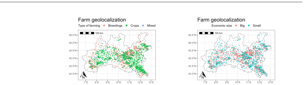
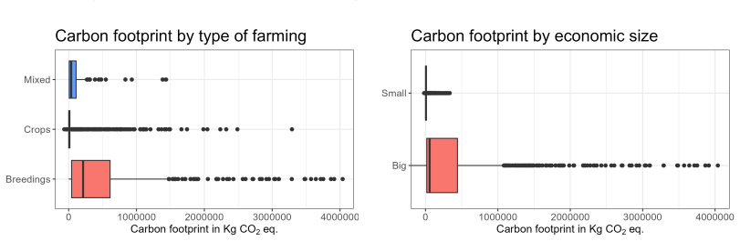
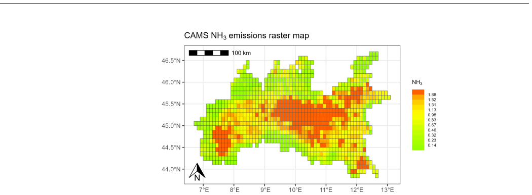
The agricultural sector is undergoing rapid change due to climate pressures, demographic shifts, and uneven economic development, increasing the demand for reliable environmental indicators at fine spatial scales. However, limited data availability often constrains subregional analyses. This study develops a model-based framework for producing reliable small-area estimates for assessing the agricultural carbon footprint in the Po Valley (Northern Italy), a region characterized by intensive livestock farming and high environmental pressure. We integrate survey, census, and satellite-derived emission data into a unified framework and produce estimates at the level of Agrarian Subregions, defined as agriculturally homogeneous municipalities by the Italian National Institute of Statistics. Satellite-based ammonia emission data are incorporated as auxiliary covariates to improve precision and spatial coherence. A key methodological contribution is the treatment of spatial misalignment between gridded satellite data and administrative boundaries. This issue is addressed through a geostatistical upscaling procedure combined with a parametric bootstrap that propagates uncertainty from the covariate construction stage to the final small-area estimates. The results show that satellite-derived information substantially improves the accuracy and stability of carbon footprint estimates while reducing reliance on large, heterogeneous auxiliary datasets, illustrating the potential of Earth observation data in model-based environmental statistics.
Editorial analysis
A structured set of objections, weighed in public.
Referee Report
Summary. This paper develops a model-based small-area estimation approach for agricultural carbon footprint in the Po Valley region of Italy. It integrates traditional survey and census data with satellite-derived ammonia emission data as auxiliary covariates, using a geostatistical upscaling procedure to address spatial misalignment between gridded satellite data and administrative boundaries, along with a parametric bootstrap to propagate uncertainty. The authors claim that this integration leads to more accurate and stable estimates at the Agrarian Subregion level while decreasing reliance on large heterogeneous auxiliary datasets.
Significance. Should the quantitative improvements be demonstrated, the work would be significant for the field of environmental statistics and small-area estimation. It highlights the potential of satellite data to enhance precision in policy-relevant indicators for agriculture under climate pressures, offering a framework that could reduce the need for extensive ground-based data collection. The combination of geostatistical methods with small-area models and uncertainty propagation is a notable methodological contribution.
major comments (3)
- [Abstract] The assertion that satellite-derived information substantially improves accuracy and stability lacks any accompanying quantitative evidence, such as comparisons of mean squared error, bias, or cross-validation results between models with and without satellite covariates. This is central to validating the paper's main contribution.
- [Methods section on covariate construction] The treatment of ammonia (NH3) satellite data as a proxy for agricultural carbon footprint (encompassing CO2, CH4, N2O) requires justification, as the link is indirect through sources like livestock and soil processes. Without reported correlations or diagnostics at the subregion scale, the improvement claim risks being driven by the specific choice of covariate rather than a robust relationship.
- [Parametric bootstrap description] While the parametric bootstrap is intended to propagate uncertainty from the geostatistical upscaling of gridded data to administrative units, it is unclear from the description whether this procedure fully incorporates potential misspecification error in the NH3 proxy or only sampling variability in the upscaling step.
minor comments (2)
- The abstract would benefit from specifying the small-area model employed (e.g., whether it is a linear mixed model or Fay-Herriot type) to provide context for the integration.
- Ensure that all acronyms (e.g., GHG, NH3) are defined at first use in the main text.
Simulated Author's Rebuttal
We thank the referee for the constructive and detailed comments, which help strengthen the manuscript. We address each major comment below and describe the planned revisions.
read point-by-point responses
-
Referee: [Abstract] The assertion that satellite-derived information substantially improves accuracy and stability lacks any accompanying quantitative evidence, such as comparisons of mean squared error, bias, or cross-validation results between models with and without satellite covariates. This is central to validating the paper's main contribution.
Authors: We agree that the abstract would be strengthened by including quantitative evidence. The results section already contains direct comparisons (including MSE reductions and cross-validation metrics) between the model with and without the satellite covariates. We will revise the abstract to report these specific improvements explicitly. revision: yes
-
Referee: [Methods section on covariate construction] The treatment of ammonia (NH3) satellite data as a proxy for agricultural carbon footprint (encompassing CO2, CH4, N2O) requires justification, as the link is indirect through sources like livestock and soil processes. Without reported correlations or diagnostics at the subregion scale, the improvement claim risks being driven by the specific choice of covariate rather than a robust relationship.
Authors: The choice of NH3 is justified by its established role as an indicator of intensive agricultural activity (livestock and fertilizer use) that drives both ammonia emissions and the greenhouse gas components of the carbon footprint in the study region. We will expand the methods section with supporting literature references and add reported correlations plus basic diagnostics between the NH3 covariate and the carbon footprint indicators at the agrarian subregion level. revision: yes
-
Referee: [Parametric bootstrap description] While the parametric bootstrap is intended to propagate uncertainty from the geostatistical upscaling of gridded data to administrative units, it is unclear from the description whether this procedure fully incorporates potential misspecification error in the NH3 proxy or only sampling variability in the upscaling step.
Authors: The parametric bootstrap as currently implemented propagates only the sampling variability associated with the geostatistical upscaling of the gridded NH3 data to administrative boundaries. It does not incorporate potential misspecification error in the NH3 proxy relationship itself. We will revise the methods description to clarify this scope and add a brief discussion of this as a methodological limitation. revision: yes
Circularity Check
No significant circularity in derivation chain
full rationale
The paper describes a standard model-based small-area estimation approach that combines survey/census data with satellite-derived ammonia emissions as auxiliary covariates, using geostatistical upscaling to handle spatial misalignment and a parametric bootstrap to propagate uncertainty from covariate construction. The reported accuracy gains are presented as empirical outcomes from comparing models with and without the satellite information, which constitutes an independent evaluation against external benchmarks rather than a reduction to fitted parameters or self-referential quantities by construction. No load-bearing self-citations, uniqueness theorems, or ansatzes are invoked in the provided text, and the central claims rest on the application of established geostatistical and SAE techniques to independent data sources without definitional equivalence between inputs and outputs.
Axiom & Free-Parameter Ledger
free parameters (1)
- small-area model parameters
axioms (2)
- domain assumption Satellite ammonia emission data correlates sufficiently with agricultural carbon emissions to serve as an effective auxiliary covariate
- domain assumption Geostatistical upscaling can align gridded satellite data to irregular administrative boundaries without substantial bias
Reference graph
Works this paper leans on
-
[1]
Ali, A., Ahmad, M., Nawaz, M., and Sattar, F. (2025). Identifying and prioritizing spatial data required for effective agriculture policymaking: A comprehensive analysis using 20/30 analytical hierarchy process.Data Intelligence, 7(1):185–220. Auteri et al.,
2025
-
[2]
Auteri, D., Attardo, C., Berzi, M., Dorati, C., Albinola, F., Baggio, L., Bucciarelli, G., Bussolari, I., and Dijkstra, L. (2024). The annual regional database of the european commission (ardeco): Methodological note. Report, JRC Working Papers on Territorial Modelling and Analysis. Baldoni et al.,
2024
-
[3]
Baldoni, E., Coderoni, S., and Esposti, R. (2017). The productivity and environment nexus with farm-level data. the case of carbon footprint in lombardy fadn farms. Bio-based and Applied Economics, 6(2):119–137. Baldoni et al.,
2017
-
[4]
Baldoni, E., Coderoni, S., and Esposti, R. (2018). The complex farm-level relationship between environmental performance and productivity: The case of carbon footprint of lombardy farms.Environmental Science & Policy, 89:73–82. Banca Dati RICA,
2018
-
[5]
Battagliese et al.,
Banca Dati RICA (2024).Sistema Documentale RICA. Battagliese et al.,
2024
-
[6]
Battagliese, D., Pollice, A., Intini, M., and Bergantino, A. S. (2026). Downscaling direct estimators in small area models.Statistical Methods & Applications, pages 1–17. Belmonte et al.,
2026
-
[7]
Belmonte, A., Riefolo, C., Buttafuoco, G., and Castrignan` o, A. (2025). An approach for spatial statistical modelling remote sensing data of land cover by fusing data of different types.Remote Sensing, 17(1):123. Bishop et al.,
2025
-
[8]
M., Fienberg, S
Bishop, Y. M., Fienberg, S. E., and Holland, P. W. (2007).Discrete multivariate analysis: Theory and practice. Springer Science & Business Media. Cameletti et al.,
2007
-
[9]
Cameletti, M., G´ omez-Rubio, V., and Blangiardo, M. (2019). Bayesian modelling for spatially misaligned health and air pollution data through the inla-spde approach. Spatial Statistics, 31:100353. CAMS,
2019
-
[10]
Carillo et al.,
CAMS (2023).CAMS2-61: Global and European emission inventories - Documentation of CAMS emission inventory products. Carillo et al.,
2023
-
[11]
C., and Salvatore, R
Carillo, F., Maranzano, P., Marcis, L., Pagliarella, M. C., and Salvatore, R. (2024). The spatio-temporal fay-herriot model using the state-space method: an application to italian lombard agrarian sub-regions.Book of Short Papers - 2nd Italian Conference on Economic Statistics (ICES
2024
-
[12]
Chi, G., Fang, H., Chatterjee, S., and Blumenstock, J. E. (2022). Microestimates of wealth for all low-and middle-income countries.Proceedings of the National Academy of Sciences, 119(3):e2113658119. Chiles and Delfiner,
2022
-
[13]
and Delfiner, P
Chiles, J.-P. and Delfiner, P. (2012).Geostatistics: Modeling Spatial Uncertainty. Wiley, Hoboken, NJ, 2nd edition. Coderoni et al.,
2012
-
[14]
Coderoni, S., Bonati, G., Longhitano, D., Papaleo, A., and Vanino, S. (2013). Impronta carbonica aziende agricole italiane. Coderoni and Esposti,
2013
-
[15]
and Esposti, R
Coderoni, S. and Esposti, R. (2018). Cap payments and agricultural ghg emissions in italy. a farm-level assessment.Science of The Total Environment, 627:427–437. Coderoni et al.,
2018
-
[16]
Coderoni, S., Esposti, R., and Baldoni, E. (2016). The productivity and environment nexus through farm-level data. the case of carbon footprint applied to lombardy fadn farms. InSeventh International Conference on Agricultural Statistics (ICAS VII), Roma, Italy, pages 26–28. Coderoni and Pagliacci,
2016
-
[17]
and Pagliacci, F
Coderoni, S. and Pagliacci, F. (2023). The impact of climate change on land productivity. a micro-level assessment for italian farms.Agricultural Systems, 205:103565. 21/30 Coderoni and Vanino,
2023
-
[18]
and Vanino, S
Coderoni, S. and Vanino, S. (2022). The farm-by-farm relationship among carbon productivity and economic performance of agriculture.Science of The Total Environment, 819:153103. Colombo et al.,
2022
-
[19]
L., Pillon, S., and Lanzani, G
Colombo, L., Marongiu, A., Malvestiti, G., Fossati, G., Angelino, E., Lazzarini, M., Gurrieri, G. L., Pillon, S., and Lanzani, G. G. (2023). Assessing the impacts and feasibility of emissions reduction scenarios in the po valley.Frontiers in Environmental Science,
2023
-
[20]
and Coderoni, S
Cortignani, R. and Coderoni, S. (2022). The impacts of environmental and climate targets on agriculture: Policy options in italy.Journal of Policy Modeling, 44(6):1095–1112. Dowd and Pardo-Ig´ uzquiza,
2022
-
[21]
Dowd, P. A. and Pardo-Ig´ uzquiza, E. (2024). The many forms of co-kriging: a diversity of multivariate spatial estimators.Mathematical Geosciences, 56(2):387–413. Edochie et al.,
2024
-
[22]
L., Ouedraogo, A., Sanoh, A., and Savadogo, A
Edochie, I., Newhouse, D., Tzavidis, N., Schmid, T., Foster, E., Hernandez, A. L., Ouedraogo, A., Sanoh, A., and Savadogo, A. (2025). Small area estimation of poverty in four west african countries by integrating survey and geospatial data.Journal of Official Statistics, 41(1):96–124. EUROSTAT, 2024a. EUROSTAT (2024a).NUTS - Nomenclature of territorial un...
2025
-
[23]
Fass` o et al., 2023.Fass` o, A., Rodeschini, J., Moro, A
EUROSTAT (2025).Animal populations by NUTS 2 regions. Fass` o et al., 2023.Fass` o, A., Rodeschini, J., Moro, A. F., Shaboviq, Q., Maranzano, P., Cameletti, M., Finazzi, F., Golini, N., Ignaccolo, R., and Otto, P. (2023). Agrimonia: a dataset on livestock, meteorology and air quality in the lombardy region, italy.Scientific Data, 10(1):143. Fay and Herriot,
2025
-
[24]
Fay, R. E. and Herriot, R. A. (1979). Estimates of income for small places: An application of james-stein procedures to census data.Journal of the American Statistical Association, 74(366a):269–277. Gardini et al.,
1979
-
[25]
Gardini, A., De Nicol` o, S., and Fabrizi, E. (2025). A mixture-of-experts model to deal with the rural/urban dichotomy in small area estimation.Journal of the Royal Statistical Society Series C: Applied Statistics, 74(5):1255–1278. Georgakis et al.,
2025
-
[26]
E., and Stamatellos, G
Georgakis, A., Papageorgiou, V. E., and Stamatellos, G. (2023). Bivariate fay-herriot model for enhanced small area estimation of growing stock volume. In2023 International Conference on Applied Mathematics & Computer Science (ICAMCS), pages 162–168. Georgakis et al.,
2023
-
[27]
E., and Stamatellos, G
Georgakis, A., Papageorgiou, V. E., and Stamatellos, G. (2024). A new approach to small area estimation: improving forest management unit estimates with advanced preprocessing in a multivariate fay–herriot model.Forestry: An International Journal of Forest Research. Gotway and Young,
2024
-
[28]
Gotway, C. A. and Young, L. J. (2002). Combining incompatible spatial data.Journal of the American Statistical Association, 97(458):632–648. Haining,
2002
-
[29]
(1990).Spatial data analysis in the social and environmental sciences
Haining, R. (1990).Spatial data analysis in the social and environmental sciences. Cambridge , MA: Cambridge University. Harmening et al.,
1990
-
[30]
Harmening, S., Kreutzmann, A.-K., Schmidt, S., Salvati, N., and Schmid, T. (2023). A framework for producing small area estimates based on area-level models in r.The R Journal, 15:316–341. https://doi.org/10.32614/RJ-2023-039. 22/30 Hassouna et al.,
-
[31]
J., Beltran, I., Amon, B., Alfaro, M
Hassouna, M., van der Weerden, T. J., Beltran, I., Amon, B., Alfaro, M. A., Anestis, V., Cinar, G., Dragoni, F., Hutchings, N. J., Leytem, A., Maeda, K., Maragou, A., Misselbrook, T., Noble, A., Rych la, A., Salazar, F., and Simon, P. (2023). Dataman: A global database of methane, nitrous oxide, and ammonia emission factors for livestock housing and outdo...
2023
-
[32]
Roma, Italy
ISTAT (2006).Regione Agraria. Roma, Italy. ISTAT,
2006
-
[33]
Kercuku et al.,
ISTAT (2020).Tavole regionali censimento dell’agricoltura. Kercuku et al.,
2020
-
[34]
Kercuku, A., Curci, F., Lanzani, A., and Zanfi, F. (2023). Italia di mezzo: The emerging marginality of intermediate territories between metropolises and inner areas.REGION, 10(1):89–112. Kreutzmann et al.,
2023
-
[35]
Kreutzmann, A.-K., Pannier, S., Rojas-Perilla, N., Schmid, T., Templ, M., and Tzavidis, N. (2019). The R package emdi for estimating and mapping regionally disaggregated indicators.Journal of Statistical Software, 91(7):1–33. Maranzano et al.,
2019
-
[36]
S., Otto, P., and Carillo, F
Maranzano, P., McConville, K. S., Otto, P., and Carillo, F. (2023). A geostatistical investigation of the ammonia-livestock relationship in the po valley, italy.Book of the Short Papers SIS 2023, pages 200–205. Marongiu et al.,
2023
-
[37]
Marongiu, A., Angelino, E., Moretti, M., Malvestiti, G., and Fossati, G. (2022). Atmospheric emission sources in the po-basin from the life-ip prepair project.Open Journal of Air Pollution, 11(3):70–83. Marongiu et al.,
2022
-
[38]
G., Distefano, G
Marongiu, A., Collalto, A. G., Distefano, G. G., and Angelino, E. (2024). Application of machine learning to estimate ammonia atmospheric emissions and concentrations.Air, 2(1):38–60. Morales et al.,
2024
-
[39]
(2021).A Course on Small Area Estimation and Mixed Models
Morales, D., Esteban, M., P´ erez, A., and Hobza, T. (2021).A Course on Small Area Estimation and Mixed Models. Springer. Newhouse et al.,
2021
-
[40]
Newhouse, D., Ramakrishnan, A., Swartz, T., Merfeld, J., and Lahiri, P. (2025). Small area estimation of monetary poverty in mexico using satellite imagery and machine learning.Oxford Bulletin of Economics and Statistics. Otto et al.,
2025
-
[41]
Otto, P., Fusta Moro, A., Rodeschini, J., Shaboviq, Q., Ignaccolo, R., Golini, N., Cameletti, M., Maranzano, P., Finazzi, F., and Fass` o, A. (2024). Spatiotemporal modelling of pm2.5 concentrations in lombardy (italy): a comparative study.Environmental and Ecological Statistics,
2024
-
[42]
Pebesma, E. J. (2004). Multivariable geostatistics in s: the gstat package.Computers & Geosciences, 30(7):683–691. Permatasari and Ubaidillah,
2004
-
[43]
and Ubaidillah, A
Permatasari, N. and Ubaidillah, A. (2025). Small area estimation of poverty using remote sensing data.Statistical Journal of the IAOS, 41(1):180–190. Pratesi and Salvati,
2025
-
[44]
and Salvati, N
Pratesi, M. and Salvati, N. (2008). Small area estimation: the eblup estimator based on spatially correlated random area effects.Statistical methods and applications, 17:113–141. Raffaelli et al.,
2008
-
[45]
Raffaelli, K., Deserti, M., Stortini, M., Amorati, R., Vasconi, M., and Giovannini, G. (2020). Improving air quality in the po valley, italy: Some results by the life-ip-prepair project.Atmosphere, 11(4):429. Rao and Molina,
2020
-
[46]
Rao, J. N. K. and Molina, I. (2015).Small Area Estimation. Wiley, New York. 23/30 Rash et al.,
2015
-
[47]
Rash, A. J. H., Khodakarami, L., Muhedin, D. A., Hamakareem, M. I., and Ali, H. F. H. (2024). Spatial modeling of geotechnical soil parameters: Integrating ground-based data, rs technique, spatial statistics and gwr model.Journal of Engineering Research, 12(1):75–85. Rawat et al.,
2024
-
[48]
Rawat, P., Kumar, M., and Airon, A. (2025). Hierarchical bayes small area estimation for rice yield using remote sensing data.Model Assisted Statistics and Applications, 20(1):52–62. Rodeschini et al.,
2025
-
[49]
Rodeschini, J., Fass` o, A., Finazzi, F., and Fusta Moro, A. (2024). Scenario analysis of livestock-related pm2.5 pollution based on a new heteroskedastic spatiotemporal model. Socio-Economic Planning Sciences, page 102053. Sabater,
2024
-
[50]
(2019).ERA5-Land hourly data from 1950 to present
Sabater, M. (2019).ERA5-Land hourly data from 1950 to present. Copernicus Climate Change Service (C3S) Climate Data Store (CDS). (Accessed on 15-05-2025),. Shawky et al.,
2019
-
[51]
A., Saad, A., and Elayouty, A
Shawky, S. A., Saad, A., and Elayouty, A. (2025). A spatial and spatiotemporal statistical downscaling model for combining spatially misaligned maximum temperature data using r-inla.Environmetrics, 36(8):e70053. Singh et al.,
2025
-
[52]
B., Shukla, G
Singh, B. B., Shukla, G. K., and Kundu, D. (2005). Spatio-temporal models in small area estimation.Survey Methodology, 31(2):183. Slud and Maiti,
2005
-
[53]
Slud, E. V. and Maiti, T. (2006). Mean-squared error estimation in transformed fay–herriot models.Journal of the Royal Statistical Society Series B: Statistical Methodology, 68(2):239–257. Tzavidis,
2006
-
[54]
Tzavidis, N. (2025). Small area estimation in the era of machine learning and alternative data sources: Opportunities, challenges, and outlook.Journal of Official Statistics, 41(3):921–929. Villejo et al.,
2025
-
[55]
J., Illian, J
Villejo, S. J., Illian, J. B., and Swallow, B. (2023). Data fusion in a two-stage spatio-temporal model using the inla-spde approach.Spatial Statistics, 54:100744. Wang et al.,
2023
-
[56]
Wang, H., Zhao, Z., Winiwarter, W., Bai, Z., Wang, X., Fan, X., Zhu, Z., Hu, C., and Ma, L. (2021). Strategies to reduce ammonia emissions from livestock and their cost-benefit analysis: A case study of sheyang county.Environmental Pollution, 290:118045. Wang et al.,
2021
-
[57]
Wang, J., Wang, Y., Li, G., and Qi, Z. (2024). Integration of remote sensing and machine learning for precision agriculture: a comprehensive perspective on applications.Agronomy, 14(9):1975. Western et al.,
2024
-
[58]
M., Sha, Z., Rigby, M., Ganesan, A
Western, L. M., Sha, Z., Rigby, M., Ganesan, A. L., Manning, A. J., Stanley, K. M., O’Doherty, S. J., Young, D., and Rougier, J. (2020). Bayesian spatio-temporal inference of trace gas emissions using an integrated nested laplacian approximation and gaussian markov random fields.Geoscientific Model Development, 13(4):2095–2107. Whittle,
2020
-
[59]
Whittle, P. (1954). ON STATIONARY PROCESSES IN THE PLANE.Biometrika, 41(3-4):434–449. Wieczorek,
1954
- [60]
-
[61]
E., Kelleghan, D
Wyer, K. E., Kelleghan, D. B., Blanes-Vidal, V., Schauberger, G., and Curran, T. P. (2022). Ammonia emissions from agriculture and their contribution to fine particulate matter: A review of implications for human health.Journal of Environmental Management, 323:116285. Ybarra and Lohr,
2022
-
[62]
Ybarra, L. M. and Lohr, S. L. (2008). Small area estimation when auxiliary information is measured with error.Biometrika, 95(4):919–931. 24/30 Zhao et al.,
2008
-
[63]
Zhao, Q., Yu, L., Du, Z., Peng, D., Hao, P., Zhang, Y., and Gong, P. (2022). An overview of the applications of earth observation satellite data: impacts and future trends.Remote Sensing, 14(8):1863. 25/30 Appendix A: Comparison between Fay-Herriot model with independent random effects and with spatially-correlated random effects To assess the efficacy of...
2022
discussion (0)
Sign in with ORCID, Apple, or X to comment. Anyone can read and Pith papers without signing in.