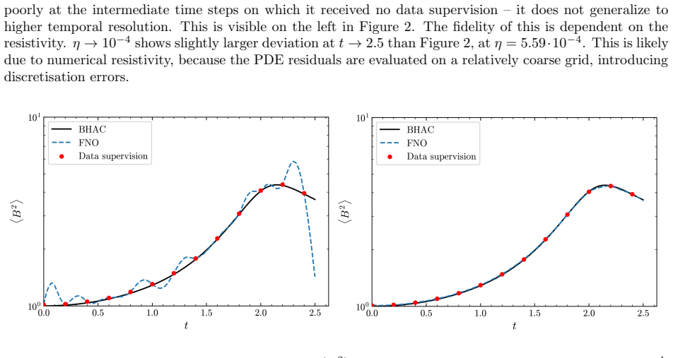
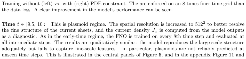
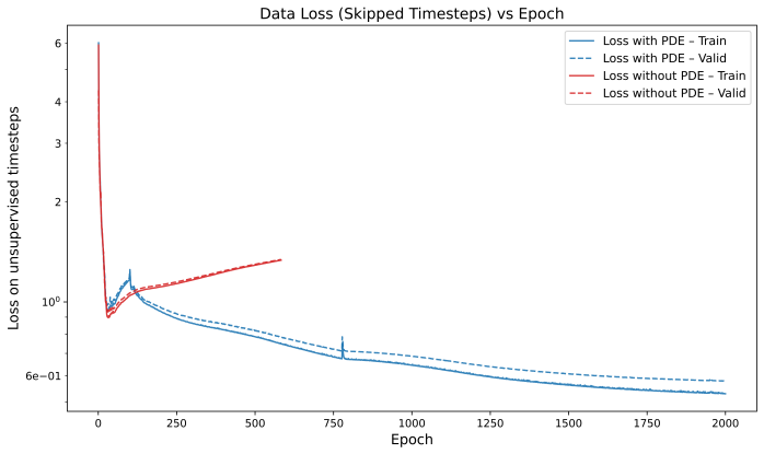
arxiv: 2604.25985 · v1 · submitted 2026-04-28 · 🌌 astro-ph.HE · cs.LG

Recognition: unknown

Learning Neural Operator Surrogates for the Black Hole Accretion Code

Cedric B\"os, Chester Tan, Christian M. Fromm, Ingo Scholtes, Karl Mannheim, Matthias N\"agele

Pith reviewed 2026-05-07 15:24 UTC · model grok-4.3

classification 🌌 astro-ph.HE cs.LG

keywords neural operatorsphysics-informed neural networksrelativistic magnetohydrodynamicsplasmoid formationmagnetic reconnectionsurrogate modelsblack hole accretionadaptive mesh refinement

0 comments

The pith

Embedding the governing equations as a loss term at finer time steps lets a neural operator recover plasmoid formation in relativistic MHD from sparse data.

A machine-rendered reading of the paper's core claim, the machinery that carries it, and where it could break.

The paper shows how neural operator models can act as fast surrogates for expensive black hole accretion simulations. A physics-informed Fourier neural operator is trained on special-relativistic resistive MHD data for the Orszag-Tang vortex, with the equations added to the loss and evaluated at finer temporal steps than the training snapshots. This lets the model learn dynamics at times without data and correctly form plasmoids during reconnection, unlike a data-only version on the same inputs. A transformer neural operator is also trained on relativistic jet simulations directly on adaptive meshes, capturing early evolution details. These are presented as the first such applications in this setting.

Core claim

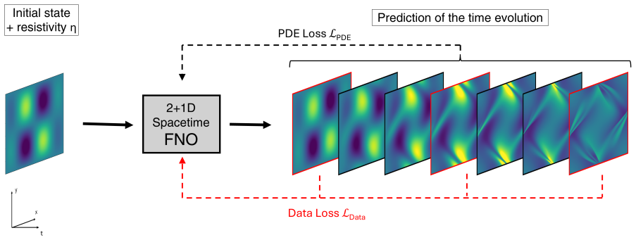
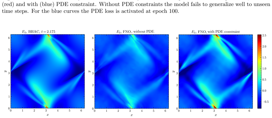
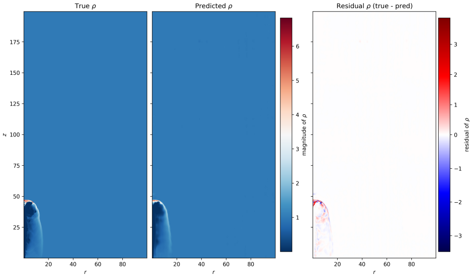
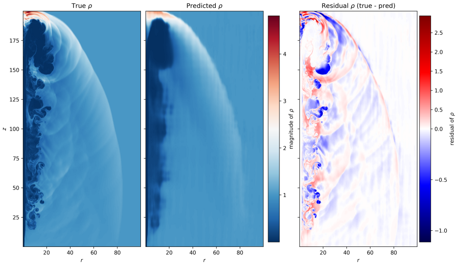
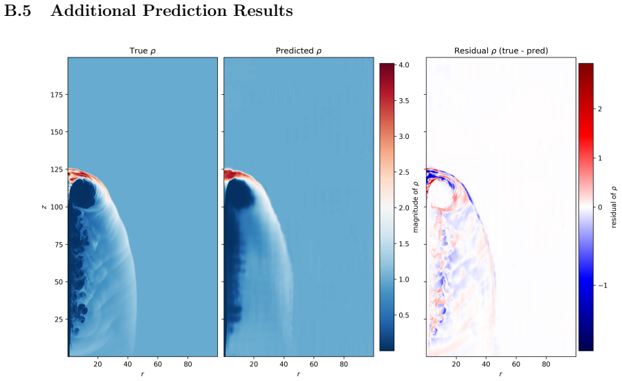
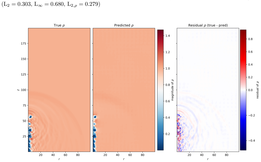
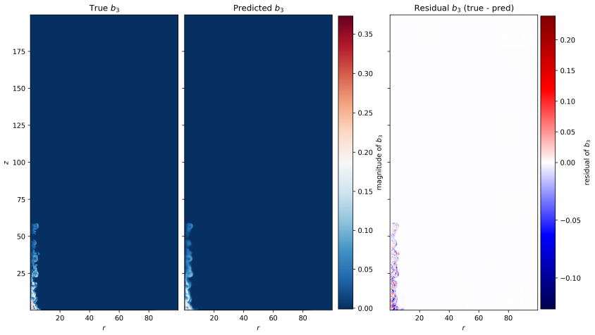
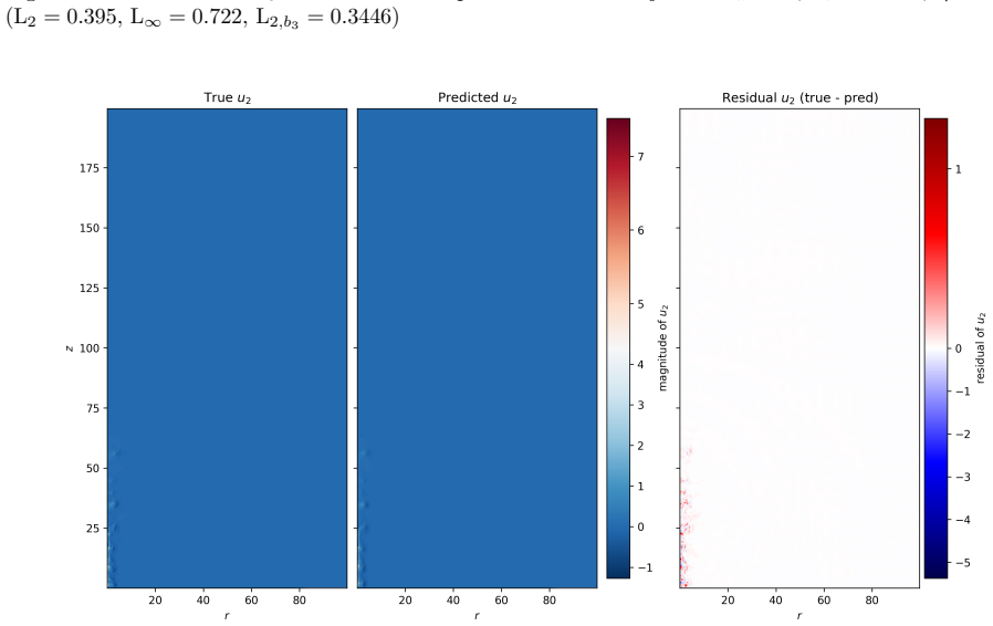
By training a Physics Informed Fourier Neural Operator on sparse snapshots of the Orszag-Tang vortex in special-relativistic resistive MHD while adding the governing equations as a loss term evaluated at finer time resolution, the surrogate learns to predict the formation of plasmoids that a data-only baseline cannot recover from the same data. This holds across a range of resistivities covering different reconnection regimes. Separately, an OFormer-style transformer neural operator applied directly to adaptive mesh refinement data from spine-sheath jet simulations reproduces major features of the evolution, particularly at early times.

What carries the argument

The physics-informed loss term from the SRRMHD equations evaluated at finer temporal resolution than the data supervision, which enables learning of intermediate dynamics.

Load-bearing premise

That enforcing the known equations at finer time steps is enough for the model to generalize to new resistivities and maintain accuracy over long times without extra constraints.

What would settle it

Running the trained PINO on a resistivity outside the training range and checking if it still correctly forms plasmoids as seen in a full simulation at that resistivity.

Figures

Figures reproduced from arXiv: 2604.25985 by Cedric B\"os, Chester Tan, Christian M. Fromm, Ingo Scholtes, Karl Mannheim, Matthias N\"agele.

**Figure 1.** Figure 1: Illustration of the used setup. The Fourier Neural Operator (FNO) received an initial state and view at source ↗

**Figure 2.** Figure 2: Domain averaged magnetic energy density ⟨B2 ⟩ as a function of time at a resistivity of η = 5.59·10−4 . Training without (left) vs. with (right) PDE constraint. The are enforced on an 8 times finer time-grid than the data loss. A clear improvement in the model’s performance can be seen. Time t ∈ [9.5, 10]: This is plasmoid regime. The spatial resolution is increased to 5122 to better resolve the fine struc… view at source ↗

**Figure 12.** Figure 12: 4.6.2 Physics Informed Training The most stable method for introducing the PDE loss was found to be as follows. The model is trained with purely data supervision for 100 epochs. Then the PDE loss weight is increased linearly with the epoch count, with the growth rate stepping up at epochs [500, 700, 1100]. Time t ∈ [0, 2.5]: The PDE loss is applied at a finer temporal resolution. The data supervision from… view at source ↗

**Figure 3.** Figure 3: The relative L2-loss (evaluated on BHAC data) on the time steps without data supervision, without (red) and with (blue) PDE constraint. Without PDE constraints the model fails to generalize well to unseen time steps. For the blue curves the PDE loss is activated at epoch 100 view at source ↗

**Figure 4.** Figure 4: Electric field Ez at a timestep without data supervision. Ground truth (left), the model’s interpolation without PDE constraints (middle) and the model’s predictions with PDE constraints enforced (right). Including the PDE loss helps the model make better predictions Time t ∈ [9.5, 10]: Again the PDE loss is enforced on a 8× finer time mesh than the data. A clear improvement is visible in view at source ↗

**Figure 5.** Figure 5: Electric current density Jz at a representative timestep without data supervision. η = 1.08 · 10−4 . Ground truth (left), the model’s interpolation without PDE constraints (middle) and the model’s predictions with PDE constraints enforced (right). Plasmoids are visible in the physics informed model, that were not present in the model without physics information. 4.7 Discussion This work demonstrates that i… view at source ↗

**Figure 6.** Figure 6: Evolving L2 error of the OFormer on the test set. After low initial errors, the model starts to produce worse predictions for later timesteps when finer details are missed. These metrics are calculated on the 27 test simulations. Looking at an early prediction of ρ shown in view at source ↗

**Figure 7.** Figure 7: Prediction of ρ at an early timestep (t = 5). The parameters for the jet are dk = 4, vb = 0.995, η = 0.006. All major details are successfully reconstructed including the top shockwave, while finer details like swirls cannot be recreated perfectly. (L2 = 0.212, L∞ = 0.697, L2,ρ = 0.185) In contrast, later predictions of ρ as shown in view at source ↗

**Figure 8.** Figure 8: Prediction of ρ at a later timestep (t = 40). The parameters for the jet are dk = 4, vb = 0.995, η = 0.006. Major details are mostly reconstructed while some finer details are missing or oversmoothed. (L2 = 0.366, L∞ = 0.729, L2,ρ = 0.396) 6 Conclusion This work presents two distinct approaches for investigating SRMHD evolution with Neural Operators. More specifically they aim at building surrogate models … view at source ↗

**Figure 9.** Figure 9: Slice of By at y = 3.129 showing the model’s performance at a timestep without data supervision, without (left) vs. with (right) PDE constraints. 18 view at source ↗

**Figure 10.** Figure 10: By from BHAC (left) with the model’s performance at a timestep without data supervision, without (middle) vs. with (right) PDE constraints. A.4.1 Plasmoid regime view at source ↗

**Figure 11.** Figure 11: Electric current density Jz at a timestep without data supervision, at resistivity η = 1.25 · 10−4 . Ground truth (left), the model’s interpolation without PDE constraints (middle) and the model’s predictions with PDE constraints enforced (right). Plasmoids are visible in the physics informed model, that were not present in the model without physics information. 19 view at source ↗

**Figure 12.** Figure 12: Electric current density Jz at a timestep without data supervision, at resistivity η = 5.59 · 10−4 . Ground truth (left), the model’s interpolation without PDE constraints (middle) and the model’s predictions with PDE constraints enforced (right). A clear improvement in accuracy is seen from the physics informed model to the model without physics information. B Details about the AMR-native Neural Operator… view at source ↗

**Figure 13.** Figure 13: Depiction of the Encoder layer (left) and Decoder layer (right) of the OFormer architecture. The view at source ↗

**Figure 14.** Figure 14: Prediction of ρ at t = 20. The parameters for the jet are dk = 4, vb = 0.995, η = 0.006. (L2 = 0.303, L∞ = 0.680, L2,ρ = 0.279) view at source ↗

**Figure 15.** Figure 15: Prediction of ρ at t = 50. The parameters for the jet are dk = 2, vb = 0.672, η = 0.002. (L2 = 0.395, L∞ = 0.722, L2,ρ = 0.2540) 24 view at source ↗

**Figure 16.** Figure 16: Prediction of b3 at t = 50. The parameters for the jet are dk = 2, vb = 0.672, η = 0.002. (L2 = 0.395, L∞ = 0.722, L2,b3 = 0.3446) view at source ↗

**Figure 17.** Figure 17: Prediction of u2 at t = 50. The parameters for the jet are dk = 2, vb = 0.672, η = 0.002. (L2 = 0.395, L∞ = 0.722, L2,u2 = 0.2091) 25 view at source ↗

read the original abstract

General-relativistic magnetohydrodynamic (GR-MHD) simulations are essential for studying black hole accretion, relativistic jets, and magnetic reconnection, yet their computational cost severely limits systematic parameter exploration. We investigate neural operator surrogates for two astrophysically relevant simulation scenarios produced by the Black Hole Accretion Code (\texttt{BHAC}). First, a Physics Informed Fourier Neural Operator (PINO) is trained on the special-relativistic resistive MHD (SRRMHD) evolution of the Orszag-Tang vortex over a range of resistivities spanning the Sweet-Parker and fast reconnection regimes. By embedding the governing equations as an additional loss term evaluated at finer temporal resolution than the available data supervision, the model learns dynamics at time steps where no simulation data is provided, enabling recovery of plasmoid formation that a data-only baseline trained on the same sparse snapshots fails to reproduce. To our knowledge, the present work is the first application of a physics informed neural operator to special relativistic resistive MHD, and the first to investigate the capability of such models to resolve plasmoid formation in SRRMHD. In a second line of investigation, an OFormer-style Transformer Neural Operator is trained on the evolution of spine-sheath relativistic jets created with \texttt{BHAC}, in special-relativistic MHD (SRMHD). The model is directly applied on the adaptive mesh, highlighting the need for linear attention due to long sequences. The neural surrogate model is capable of capturing most of the major details, especially in early predictions. To our knowledge, this constitutes the first application of a neural operator directly on a high resolution adaptive mesh refinement grid in the context of MHD simulations.

Editorial analysis

A structured set of objections, weighed in public.

Desk editor's note, referee report, simulated authors' rebuttal, and a circularity audit. Tearing a paper down is the easy half of reading it; the pith above is the substance, this is the friction.

Desk Editor's Note private letter to a colleague

The paper demonstrates a first use of physics-informed neural operators on special-relativistic resistive MHD and AMR grids for jet simulations, with qualitative gains from the physics loss on plasmoid recovery, but lacks the quantitative checks needed to confirm long-term reliability.

read the letter

The main takeaway is that this work applies PINO to SRRMHD Orszag-Tang vortex runs across resistivities and an OFormer-style operator directly to AMR data for spine-sheath jets. Both are presented as firsts in the domain, and the physics loss term evaluated at finer timesteps appears to let the model recover plasmoid formation that a pure data-driven baseline misses on the same sparse snapshots. That is a concrete, useful observation for anyone trying to stretch limited GR-MHD compute budgets. The AMR handling with linear attention is also a practical step for real simulation outputs rather than uniform grids. Credit is due for shipping the approach on actual BHAC data instead of toy problems. The manuscript stays grounded in the governing equations and does not overclaim universality. The soft spots sit mainly in the evaluation. The abstract and available description give no L2 residuals, growth-rate comparisons, or long-horizon rollout errors, so it is hard to judge whether the physics loss actually prevents accumulation or just delays it. Generalization to resistivities outside the training interval is asserted but not quantified with held-out tests or stability metrics. If those numbers are weak or absent in the full text, the central claim about learning unseen dynamics rests on thinner ground than the qualitative images suggest. A reader working on surrogate modeling for accretion or reconnection will find the setup and the AMR experiment worth examining. Someone outside that niche will get less immediate value. The paper is coherent on its own terms and shows clear thinking about the inductive bias the physics term supplies, so it merits a serious referee rather than a desk reject. I would send it out for review with the expectation that the authors add the missing error tables and at least one out-of-distribution resistivity test.

Referee Report

3 major / 2 minor

Summary. The manuscript introduces neural operator surrogates for black hole accretion simulations produced by the Black Hole Accretion Code (BHAC). A Physics-Informed Fourier Neural Operator (PINO) is trained on special-relativistic resistive MHD (SRRMHD) Orszag-Tang vortex evolution across a resistivity range, embedding the governing equations as a loss term evaluated at finer temporal resolution than the training snapshots; this is claimed to recover plasmoid formation that a data-only baseline fails to reproduce. Separately, an OFormer-style transformer neural operator is trained on spine-sheath relativistic jets in special-relativistic MHD (SRMHD) and applied directly on adaptive mesh refinement grids. The work positions itself as the first application of physics-informed neural operators to SRRMHD and the first neural operator on high-resolution AMR MHD grids.

Significance. If the central claims hold, the approach could substantially accelerate parameter studies of black hole accretion, jets, and magnetic reconnection by providing fast, physics-constrained surrogates that generalize beyond sparse training data. The explicit use of SRRMHD equations in the loss and the direct handling of AMR grids represent technical novelties that, if quantitatively validated, would strengthen the case for physics-informed neural operators in relativistic astrophysics.

major comments (3)

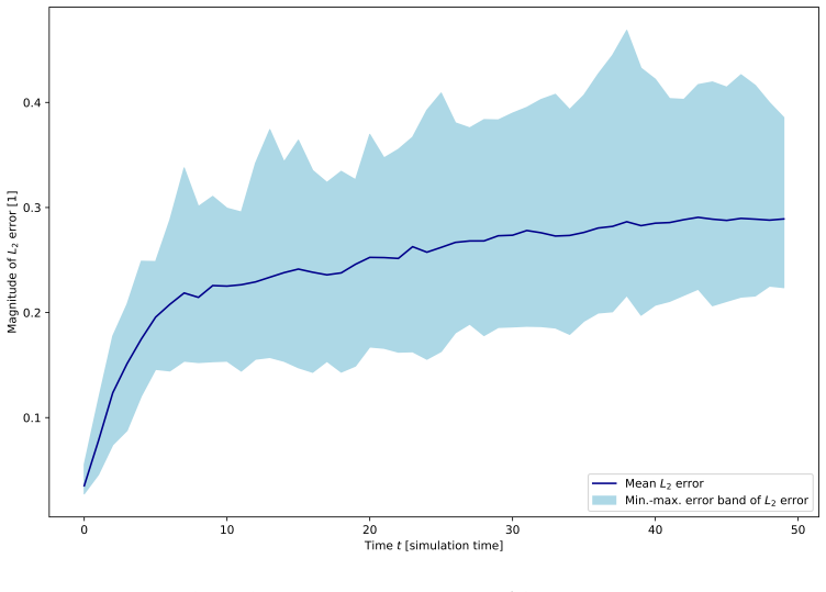
[Abstract] Abstract: The claim that embedding the SRRMHD equations as a loss at finer temporal resolution enables recovery of plasmoid formation absent from the sparse snapshots is load-bearing for the central contribution, yet the abstract (and presumably the results section) supplies no quantitative metrics such as L2 residuals on the magnetic field, plasmoid growth rates, or long-horizon rollout errors relative to the data-only baseline or full BHAC runs. Without these, the superiority cannot be assessed and the weakest assumption (stable enforcement preventing error accumulation for unseen resistivities) remains untested.
[Abstract] Abstract / Results (plasmoid section): Generalization to resistivities outside the training interval and autoregressive stability beyond the supervised horizon are asserted but not demonstrated; no ablation on resistivity range, no residual norms of the discrete SRRMHD equations at intermediate times, and no comparison of long-term evolution against reference simulations are reported. This directly affects whether the physics loss supplies sufficient inductive bias.
[Abstract] Jet section: The statement that the OFormer 'captures most of the major details, especially in early predictions' on the AMR grid lacks supporting quantitative evidence (e.g., pointwise or integrated error norms, conservation diagnostics, or metrics at late times). Given the emphasis on linear attention for long sequences, the absence of sequence-length scaling or stability tests for extended rollouts is a load-bearing gap for the claimed applicability to realistic jet evolution.

minor comments (2)

[Abstract] Notation for the resistivity parameter range and the precise form of the physics loss term should be defined explicitly (including how the finer temporal collocation points are chosen) to allow reproducibility.
The manuscript should include a brief comparison to prior neural operator applications in MHD (e.g., standard FNO or DeepONet baselines) to clarify the incremental benefit of the physics-informed and AMR-specific choices.

Simulated Author's Rebuttal

3 responses · 0 unresolved

We thank the referee for their constructive and detailed report. The comments highlight important gaps in quantitative validation that we agree need to be addressed to strengthen the manuscript. We respond point-by-point below and will incorporate all suggested additions in the revised version.

read point-by-point responses

Referee: [Abstract] Abstract: The claim that embedding the SRRMHD equations as a loss at finer temporal resolution enables recovery of plasmoid formation absent from the sparse snapshots is load-bearing for the central contribution, yet the abstract (and presumably the results section) supplies no quantitative metrics such as L2 residuals on the magnetic field, plasmoid growth rates, or long-horizon rollout errors relative to the data-only baseline or full BHAC runs. Without these, the superiority cannot be assessed and the weakest assumption (stable enforcement preventing error accumulation for unseen resistivities) remains untested.

Authors: We agree that quantitative metrics are essential to substantiate the superiority claim. In the revised manuscript we will add L2 residuals on the magnetic field, plasmoid growth rates, and long-horizon rollout errors relative to both the data-only baseline and full BHAC reference runs. These metrics will be presented in the results section and referenced from the abstract, directly addressing the stability of the physics-informed enforcement for unseen resistivities. revision: yes
Referee: [Abstract] Abstract / Results (plasmoid section): Generalization to resistivities outside the training interval and autoregressive stability beyond the supervised horizon are asserted but not demonstrated; no ablation on resistivity range, no residual norms of the discrete SRRMHD equations at intermediate times, and no comparison of long-term evolution against reference simulations are reported. This directly affects whether the physics loss supplies sufficient inductive bias.

Authors: We acknowledge that generalization and long-term stability require explicit demonstration. The revised version will include ablations on resistivity range, residual norms of the discrete SRRMHD equations evaluated at intermediate times, and side-by-side long-term evolution comparisons against reference BHAC simulations. These additions will quantify the inductive bias supplied by the physics loss term. revision: yes
Referee: [Abstract] Jet section: The statement that the OFormer 'captures most of the major details, especially in early predictions' on the AMR grid lacks supporting quantitative evidence (e.g., pointwise or integrated error norms, conservation diagnostics, or metrics at late times). Given the emphasis on linear attention for long sequences, the absence of sequence-length scaling or stability tests for extended rollouts is a load-bearing gap for the claimed applicability to realistic jet evolution.

Authors: We agree that the jet results require quantitative backing. The revised manuscript will report pointwise and integrated error norms, conservation diagnostics, and metrics at late times. We will additionally include sequence-length scaling behavior and stability tests for extended autoregressive rollouts to support applicability to realistic jet evolution. revision: yes

Circularity Check

0 steps flagged

No significant circularity; training uses external data plus independent known equations

full rationale

The paper trains PINO and Transformer neural operators on external BHAC simulation snapshots while adding the established SRRMHD/SRMHD governing equations as a physics loss evaluated at finer timesteps. This is not circular: the data supervision comes from independent numerical simulations, the physics loss encodes pre-existing PDEs rather than any fitted parameter or self-referential definition, and the claimed recovery of plasmoid formation is an empirical result of the combined loss rather than a reduction to the inputs by construction. No self-citation chains, uniqueness theorems, or renamed known results appear as load-bearing steps in the abstract or described methodology.

Axiom & Free-Parameter Ledger

1 free parameters · 1 axioms · 0 invented entities

Ledger is necessarily incomplete because only the abstract is available; no explicit free parameters, axioms, or invented entities are stated beyond the standard neural-operator training setup and the assumption that SRRMHD equations are known.

free parameters (1)

resistivity range
Training performed over a range of resistivities spanning Sweet-Parker and fast reconnection regimes; exact sampling points not specified.

axioms (1)

domain assumption The resistive MHD equations can be discretized and evaluated as a loss term at arbitrary time steps
Core premise enabling the physics-informed component; invoked when the model is trained on finer temporal resolution than the data.

pith-pipeline@v0.9.0 · 5622 in / 1271 out tokens · 49331 ms · 2026-05-07T15:24:36.304984+00:00 · methodology

discussion (0)

Reference graph

Works this paper leans on

58 extracted references · 32 canonical work pages · 6 internal anchors

[2]

& Yoshida, N

Event Horizon Telescope Collaboration et al. “First M87 Event Horizon Telescope Results. V. Physical Origin of the Asymmetric Ring”. In:apjl875.1, L5 (Apr. 2019), p. L5.doi:10.3847/2041- 8213/ ab0f43. arXiv:1906.11242 [astro-ph.GA]

work page doi:10.3847/2041- 2019
[3]

The Black Hole Accretion Code

O. Porth et al. “The Black Hole Accretion Code”. In:Computational Astrophysics and Cosmology4.1 (2017), p. 1.doi:10.1186/s40668- 017- 0020- 2.url:https://doi.org/10.1186/s40668- 017- 0020-2

work page doi:10.1186/s40668- 2017
[4]

Aghanimet al.[Planck], Astron

H. Olivares et al. “Constrained transport and adaptive mesh refinement in the Black Hole Accretion Code”. In:Astronomy & Astrophysics629 (2019), A61.doi:10.1051/0004- 6361/201935559.url: https://doi.org/10.1051/0004-6361/201935559

work page doi:10.1051/0004- 2019
[5]

General-relativistic Resistive Magnetohydrodynamics with Robust Primitive-variable Recovery for Accretion Disk Simulations

B. Ripperda et al. “General-relativistic Resistive Magnetohydrodynamics with Robust Primitive-variable Recovery for Accretion Disk Simulations”. In:The Astrophysical Journal Supplement Series244.1 (2019), p. 10.doi:10.3847/1538-4365/ab3922.url:https://doi.org/10.3847/1538-4365/ab3922

work page doi:10.3847/1538-4365/ab3922.url:https://doi.org/10.3847/1538-4365/ab3922 2019
[6]

2019, ApJS, 243, 26, doi: 10.3847/1538-4365/ab29fd

Oliver Porth et al. “The Event Horizon General Relativistic Magnetohydrodynamic Code Comparison Project”. In:apjs243.2, 26 (Aug. 2019), p. 26.doi:10.3847/1538-4365/ab29fd. arXiv:1904.04923 [astro-ph.HE]

work page doi:10.3847/1538-4365/ab29fd 2019
[7]

Nikola Kovachki, Zongyi L, and Burigede Liu et al.Neural Operator: Learning Maps Between Function Spaces. 2021. arXiv:2108.08481 [cs.LG].url:https://arxiv.org/abs/2108.08481

work page arXiv 2021
[8]

Zongyi Li et al.Fourier Neural Operator for Parametric Partial Differential Equations. 2021. arXiv: 2010.08895 [cs.LG].url:https://arxiv.org/abs/2010.08895

work page internal anchor Pith review arXiv 2021
[9]

Zongyi Li et al.Physics-Informed Neural Operator for Learning Partial Differential Equations. 2023. arXiv:2111.03794 [cs.LG].url:https://arxiv.org/abs/2111.03794

work page arXiv 2023
[10]

Magnetohydrodynamics with physics informed neural operators

Shawn G Rosofsky and E A Huerta. “Magnetohydrodynamics with physics informed neural operators”. In:Machine Learning: Science and Technology4.3 (June 2023), p. 035002.doi:10 . 1088 / 2632 - 2153/ace30a.url:https://doi.org/10.1088/2632-2153/ace30a

work page doi:10.1088/2632-2153/ace30a 2023
[11]

Roberta Duarte, Rodrigo Nemmen, and Reinaldo Santos-Lima.Spectral Learning of Magnetized Plasma Dynamics: A Neural Operator Application. 2025. arXiv:2507 . 01388 [astro-ph.HE].url:https : //arxiv.org/abs/2507.01388

work page arXiv 2025
[12]

Parallel, grid-adaptive approaches for relativistic hydro and magnetohydrody- namics

Rony Keppens et al. “Parallel, grid-adaptive approaches for relativistic hydro and magnetohydrody- namics”. In:Journal of Computational Physics231.3 (2012), pp. 718–744

2012
[13]

MPI-AMRVAC for solar and astrophysics

O Porth et al. “MPI-AMRVAC for solar and astrophysics”. In:The Astrophysical Journal Supplement Series214.1 (2014), p. 4. 14

2014
[14]

Solving the Orszag–Tang vortex magnetohydrodynamics problem with physics-constrained convolutional neural networks

A. Bormanis, C. A. Leon, and A. Scheinker. “Solving the Orszag–Tang vortex magnetohydrodynamics problem with physics-constrained convolutional neural networks”. In:Physics of Plasmas31.1 (Jan. 2024), p. 012101.issn: 1070-664X.doi:10 . 1063 / 5 . 0172075. eprint:https : / / pubs . aip . org / aip / pop / article - pdf / doi / 10 . 1063 / 5 . 0172075 / 1972...

work page doi:10.1063/5.0172075 2024
[15]

Resolving turbulent magnetohydrodynamics: a hy- brid operator-diffusion framework

Semih Kacmaz, E A Huerta, and Roland Haas. “Resolving turbulent magnetohydrodynamics: a hy- brid operator-diffusion framework”. In:Machine Learning: Science and Technology6.3 (Sept. 2025), p. 035057.issn: 2632-2153.doi:10.1088/2632-2153/ae054c.url:http://dx.doi.org/10.1088/ 2632-2153/ae054c

work page doi:10.1088/2632-2153/ae054c.url:http://dx.doi.org/10.1088/ 2025
[16]

Taeyoung Kim, Youngsoo Ha, and Myungjoo Kang.Neural Operators Learn the Local Physics of Mag- netohydrodynamics. 2024. arXiv:2404.16015 [physics.comp-ph].url:https://arxiv.org/abs/ 2404.16015

work page arXiv 2024
[17]

Corwin Cheung et al.Reconstructing Relativistic Magnetohydrodynamics with Physics-Informed Neural Networks. 2025. arXiv:2512.23057 [physics.comp-ph].url:https://arxiv.org/abs/2512.23057

work page arXiv 2025
[18]

Small-scale structure of two-dimensional magnetohydrodynamic turbulence

Steven A. Orszag and Cha-Mei Tang. “Small-scale structure of two-dimensional magnetohydrodynamic turbulence”. In:Journal of Fluid Mechanics90.1 (1979), pp. 129–143.doi:10.1017/S002211207900210X

work page doi:10.1017/s002211207900210x 1979
[19]

Magnetic Reconnection and Hot Spot Formation in Black Hole Accretion Disks

Bart Ripperda, Fabio Bacchini, and Alexander A. Philippov. “Magnetic Reconnection and Hot Spot Formation in Black Hole Accretion Disks”. In:The Astrophysical Journal900.2 (Sept. 2020), p. 100. issn: 1538-4357.doi:10 . 3847 / 1538 - 4357 / ababab.url:http : / / dx . doi . org / 10 . 3847 / 1538 - 4357/ababab

2020
[20]

Version 1.2.0

PhysicsNeMo Contributors.NVIDIA PhysicsNeMo: An open-source framework for physics-based deep learning in science and engineering. Version 1.2.0. Feb. 2023.url:https://github.com/NVIDIA/ physicsnemo

2023
[21]

Tim De Ryck, Siddhartha Mishra, and Roberto Molinaro.wPINNs: Weak Physics informed neural networks for approximating entropy solutions of hyperbolic conservation laws. 2022. arXiv:2207.08483 [math.NA].url:https://arxiv.org/abs/2207.08483

work page arXiv 2022
[22]

Challenges and advancements in modeling shock fronts with physics-informed neu- ral networks: A review and benchmarking study

Jassem Abbasi et al. “Challenges and advancements in modeling shock fronts with physics-informed neu- ral networks: A review and benchmarking study”. In:Neurocomputing657 (2025), p. 131440.issn: 0925- 2312.doi:https://doi.org/10.1016/j.neucom.2025.131440.url:https://www.sciencedirect. com/science/article/pii/S0925231225021125

work page doi:10.1016/j.neucom.2025.131440.url:https://www.sciencedirect 2025
[23]

INTEGRAL PINNS FOR HYPERBOLIC CON- SERVATION LAWS

Manvendra P. Rajvanshi and David I Ketcheson. “INTEGRAL PINNS FOR HYPERBOLIC CON- SERVATION LAWS”. In:ICLR 2024 Workshop on AI4DifferentialEquations In Science. 2024.url: https://openreview.net/forum?id=Uuu6HWe6dF

2024
[24]

Kharma: Flexible, portable performance for grmhd

Ben S Prather. “Kharma: Flexible, portable performance for grmhd”. In:New Frontiers in GRMHD Simulations. Springer, 2025, pp. 167–201

2025
[25]

OpenFOAM: A C++ library for complex physics simulations

Hrvoje Jasak, Aleksandar Jemcov, Zeljko Tukovic, et al. “OpenFOAM: A C++ library for complex physics simulations”. In:International workshop on coupled methods in numerical dynamics. Vol. 1000. Dubrovnik, Croatia). 2007, pp. 1–20

2007
[26]

Dynamic mesh handling in OpenFOAM

Hrvoje Jasak. “Dynamic mesh handling in OpenFOAM”. In:47th AIAA aerospace sciences meeting including the new horizons forum and aerospace exposition. 2009, p. 341

2009
[27]

Spherical fourier neural operators: Learning stable dynamics on the sphere

Boris Bonev et al. “Spherical fourier neural operators: Learning stable dynamics on the sphere”. In: International conference on machine learning. PMLR. 2023, pp. 2806–2823

2023
[28]

Computing Fourier transforms and convolutions on the 2- sphere

James R Driscoll and Dennis M Healy. “Computing Fourier transforms and convolutions on the 2- sphere”. In:Advances in applied mathematics15.2 (1994), pp. 202–250

1994
[29]

Fourier neural operator with learned deformations for pdes on general geometries

Zongyi Li et al. “Fourier neural operator with learned deformations for pdes on general geometries”. In:Journal of Machine Learning Research24.388 (2023), pp. 1–26

2023
[30]

Neural operator: Graph kernel network for partial differential equations.arXiv preprint arXiv:2003.03485, 2020

Zongyi Li et al. “Neural operator: Graph kernel network for partial differential equations”. In:arXiv preprint arXiv:2003.03485(2020). 15

work page arXiv 2003
[31]

The graph neural network model

Franco Scarselli et al. “The graph neural network model”. In:IEEE transactions on neural networks 20.1 (2008), pp. 61–80

2008
[32]

Semi-Supervised Classification with Graph Convolutional Networks

Thomas N Kipf and Max Welling. “Semi-supervised classification with graph convolutional networks”. In:arXiv preprint arXiv:1609.02907(2016)

work page internal anchor Pith review arXiv 2016
[33]

Geometry-informed neural operator for large-scale 3d pdes

Zongyi Li et al. “Geometry-informed neural operator for large-scale 3d pdes”. In:Advances in Neural Information Processing Systems36 (2023), pp. 35836–35854

2023
[34]

¨Uber die praktische Aufl¨ osung von Integralgleichungen mit Anwendungen auf Randwertaufgaben

Evert J Nystr¨ om. “ ¨Uber die praktische Aufl¨ osung von Integralgleichungen mit Anwendungen auf Randwertaufgaben”. In:Acta Mathematica(1930)

1930
[35]

Transolver-3: Scaling Up Transformer Solvers to Industrial-Scale Geometries,

Hang Zhou et al. “Transolver-3: Scaling Up Transformer Solvers to Industrial-Scale Geometries”. In: arXiv preprint arXiv:2602.04940(2026)

work page arXiv 2026
[36]

Pretraining codomain attention neural operators for solving multiphysics pdes

Ashiqur Rahman et al. “Pretraining codomain attention neural operators for solving multiphysics pdes”. In:Advances in Neural Information Processing Systems37 (2024), pp. 104035–104064

2024
[37]

Continuum attention for neural operators

Edoardo Calvello et al. “Continuum attention for neural operators”. In:Journal of Machine Learning Research26.300 (2025), pp. 1–52

2025
[38]

Attention is all you need

Ashish Vaswani et al. “Attention is all you need”. In:Advances in neural information processing systems 30 (2017)

2017
[39]

An Image is Worth 16x16 Words: Transformers for Image Recognition at Scale

Alexey Dosovitskiy et al. “An image is worth 16x16 words: Transformers for image recognition at scale”. In:arXiv preprint arXiv:2010.11929(2020)

work page internal anchor Pith review arXiv 2010
[40]

Universal physics transformers: A framework for efficiently scaling neural oper- ators

Benedikt Alkin et al. “Universal physics transformers: A framework for efficiently scaling neural oper- ators”. In:Advances in Neural Information Processing Systems37 (2024), pp. 25152–25194

2024
[41]

Mesh-informed neural operator: A transformer generative approach

Yaozhong Shi et al. “Mesh-informed neural operator: A transformer generative approach”. In:arXiv preprint arXiv:2506.16656(2025)

work page arXiv 2025
[42]

Geometry-aware operator transformer as an efficient and accurate neural surrogate for PDEs on arbitrary domains.arXiv preprint arXiv:2505.18781, 2025

Shizheng Wen et al. “Geometry aware operator transformer as an efficient and accurate neural surrogate for pdes on arbitrary domains”. In:arXiv preprint arXiv:2505.18781(2025)

work page arXiv 2025
[43]

Transolver: A Fast Transformer Solver for PDEs on General Geometries,

Haixu Wu et al. “Transolver: A fast transformer solver for pdes on general geometries”. In:arXiv preprint arXiv:2402.02366(2024)

work page arXiv 2024
[44]

Transolver++: An accurate neural solver for pdes on million-scale geometries.arXiv preprint arXiv:2502.02414, 2025

Huakun Luo et al. “Transolver++: An accurate neural solver for pdes on million-scale geometries”. In: arXiv preprint arXiv:2502.02414(2025)

work page arXiv 2025
[45]

AMR-Transformer: enabling efficient long-range interaction for complex neural fluid sim- ulation

Zeyi Xu et al. “AMR-Transformer: enabling efficient long-range interaction for complex neural fluid sim- ulation”. In:Proceedings of the Computer Vision and Pattern Recognition Conference. 2025, pp. 5804– 5813

2025
[46]

Choose a transformer: Fourier or galerkin

Shuhao Cao. “Choose a transformer: Fourier or galerkin”. In:Advances in neural information processing systems34 (2021), pp. 24924–24940

2021
[47]

Transformer for partial differential equations’ operator learning, 2023

Zijie Li, Kazem Meidani, and Amir Barati Farimani. “Transformer for partial differential equations’ operator learning”. In:arXiv preprint arXiv:2205.13671(2022)

work page arXiv 2022
[48]

Layer Normalization

Jimmy Lei Ba, Jamie Ryan Kiros, and Geoffrey E Hinton. “Layer normalization”. In:arXiv preprint arXiv:1607.06450(2016)

work page internal anchor Pith review arXiv 2016
[49]

Principled approaches for extending neural architectures to function spaces for operator learning

Julius Berner et al. “Principled approaches for extending neural architectures to function spaces for operator learning”. In:arXiv preprint arXiv:2506.10973(2025)

work page arXiv 2025
[50]

Root mean square layer normalization

Biao Zhang and Rico Sennrich. “Root mean square layer normalization”. In:Advances in neural infor- mation processing systems32 (2019)

2019
[51]

Gaussian Error Linear Units (GELUs)

Dan Hendrycks and Kevin Gimpel. “Gaussian error linear units (gelus)”. In:arXiv preprint arXiv:1606.08415 (2016)

work page internal anchor Pith review arXiv 2016
[52]

Roformer: Enhanced transformer with rotary position embedding

Jianlin Su et al. “Roformer: Enhanced transformer with rotary position embedding”. In:Neurocomput- ing568 (2024), p. 127063

2024
[53]

Neural operator: Learning maps between function spaces with applications to pdes

Nikola Kovachki et al. “Neural operator: Learning maps between function spaces with applications to pdes”. In:Journal of Machine Learning Research24.89 (2023), pp. 1–97. 16

2023
[54]

Decoupled Weight Decay Regularization

Ilya Loshchilov and Frank Hutter. “Decoupled weight decay regularization”. In:arXiv preprint arXiv:1711.05101 (2017)

work page internal anchor Pith review arXiv 2017
[55]

Paardekooper, C

Serguei S. Komissarov. “Multidimensional numerical scheme for resistive relativistic magnetohydrody- namics: Multidimensional numerical scheme for resistive relativistic MHD”. In:Monthly Notices of the Royal Astronomical Society382.3 (Nov. 2007), pp. 995–1004.issn: 0035-8711.doi:10.1111/j.1365- 2966.2007.12448.x.url:http://dx.doi.org/10.1111/j.1365-2966.2...

work page doi:10.1111/j.1365- 2007
[56]

Valentin Duruisseaux, Jean Kossaifi, and Anima Anandkumar.Fourier Neural Operators Explained: A Practical Perspective. 2026. arXiv:2512.01421 [cs.LG].url:https://arxiv.org/abs/2512.01421

work page arXiv 2026
[57]

Stationary relativistic jets

Serguei S Komissarov, Oliver Porth, and Maxim Lyutikov. “Stationary relativistic jets”. In:Computa- tional astrophysics and cosmology2.1 (2015), p. 9

2015
[58]

Radiative signatures of Parsec-Scale magnetised jets

Christian M Fromm et al. “Radiative signatures of Parsec-Scale magnetised jets”. In:Galaxies5.4 (2017), p. 73. Appendix A Details about the PINO for resistive SRMHD A.1 Special-Relativistic Resistive MHD equations Maxwell’s equations ∇ ·B= 0 (4) ∂tB+∇ ×E= 0 (5) ∇ ·E=q(6) −∂tE+∇ ×B=J(7) Ohm’s law in the general inertial frame is given by J= γ η [E+v×B−(E·v...

2017
[59]

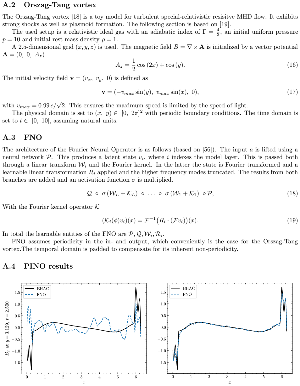
The physical domain is set to (x, y)∈[0,2π] 2 with periodic boundary conditions

This ensures the maximum speed is limited by the speed of light. The physical domain is set to (x, y)∈[0,2π] 2 with periodic boundary conditions. The time domain is set tot∈[0,10], assuming natural units. A.3 FNO The architecture of the Fourier Neural Operator is as follows (based on [56]). The inputais lifted using a neural networkP. This produces a late...

2091