arxiv: 2604.26205 · v1 · submitted 2026-04-29 · 💰 econ.EM

Recognition: unknown

Sequential Estimation of Dynamic Discrete Choice Models with Unobserved Heterogeneity

Ertian Chen , Hiroyuki Kasahara , Katsumi Shimotsu

Authors on Pith no claims yet

Pith reviewed 2026-05-07 12:41 UTC · model grok-4.3

classification 💰 econ.EM

keywords dynamic discrete choiceunobserved heterogeneityEM algorithmfixed-point iterationtruncation invariancesequential estimationlinear-in-parameters models

0 comments

The pith

Truncating the inner fixed-point solver after any number of steps leaves the EM-NPL estimator numerically identical in linear-in-parameters models.

A machine-rendered reading of the paper's core claim, the machinery that carries it, and where it could break.

The paper develops the EM-NPL(q) procedure that pairs the expectation-maximization algorithm with an inner fixed-point solver stopped after only q iterations. For the standard linear-in-parameters specification of dynamic discrete choice models, it proves that the resulting estimator is exactly the same no matter whether q equals 1 or runs to full convergence. Because the numerical value does not change, any truncation affects only the speed of computation and leaves the estimator's consistency, asymptotic normality, and local convergence properties untouched. Monte Carlo evidence shows runtime reductions of 20 percent to fivefold. An application to cola demand finds that omitting unobserved heterogeneity understates long-run own-price elasticities by as much as 60 percent, short-run elasticities by 85 percent, and the compensating variation of a soda tax by 90 percent.

Core claim

For the workhorse class of linear-in-parameters models, for any q greater than or equal to 1 the EM-NPL(q) estimator is numerically identical to the EM-NPL estimator that solves the inner fixed-point problem to convergence. The choice of q therefore influences only computational cost and not statistical properties. The estimator is consistent and asymptotically normal, and the algorithm converges locally.

What carries the argument

The truncation-invariance property of the EM-NPL(q) algorithm for linear-in-parameters dynamic discrete choice models.

If this is right

The estimator remains consistent and asymptotically normal for any fixed q greater than or equal to 1.
Local convergence of the EM-NPL(q) algorithm is guaranteed under standard conditions.
Runtime falls by at least 20 percent and can reach a factor of three to five in Monte Carlo designs.
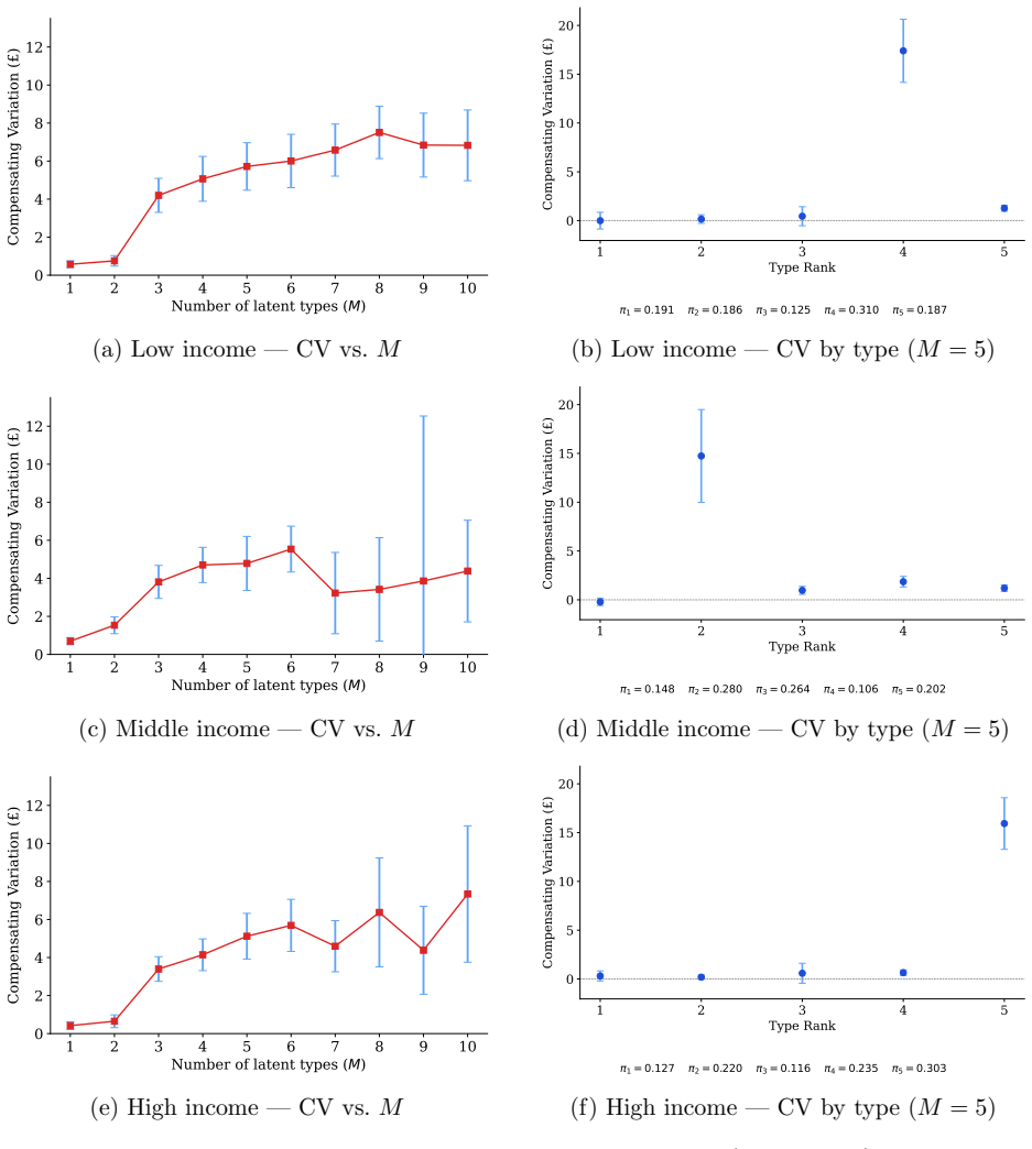
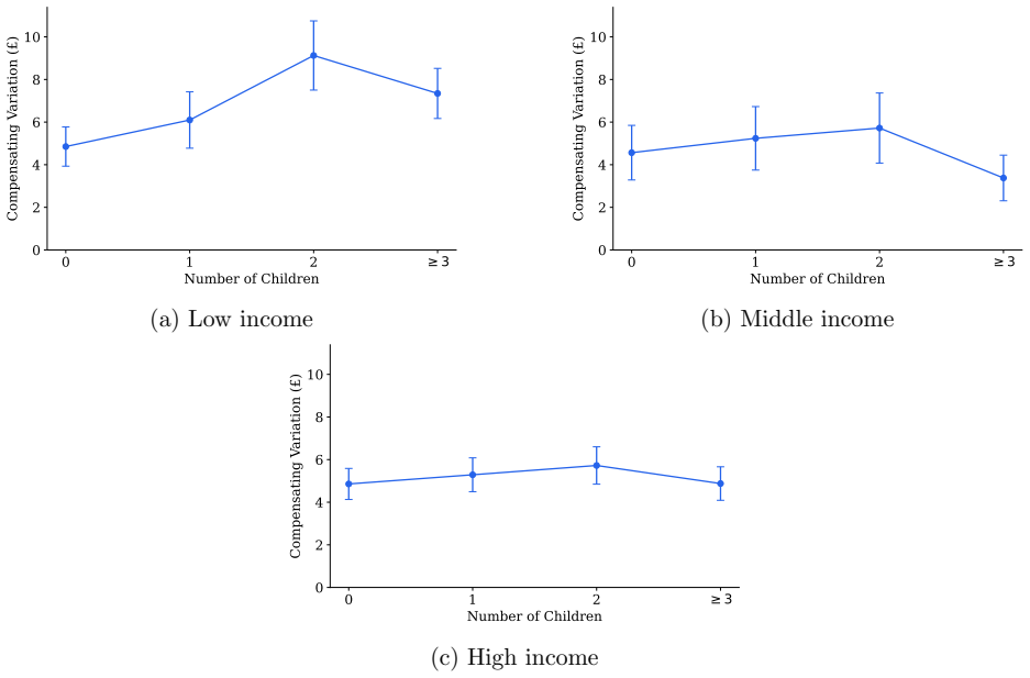
Accounting for unobserved heterogeneity raises estimated long-run own-price elasticities by up to 60 percent, short-run elasticities by up to 85 percent, and compensating variation from a soda tax by up to 90 percent.

Where Pith is reading between the lines

These are editorial extensions of the paper, not claims the author makes directly.

The invariance may allow researchers to estimate models with larger numbers of unobserved types than were previously practical.
Small fixed values of q such as 1 or 2 can be adopted without any need to verify convergence of the inner loop.
Related EM-based estimators outside dynamic discrete choice may possess analogous invariance properties that could be checked directly.

Load-bearing premise

The truncation-invariance result holds specifically for the workhorse class of linear-in-parameters models.

What would settle it

A concrete linear-in-parameters model in which the numerical value of the EM-NPL(1) estimate differs from the value obtained by solving the inner fixed-point problem to convergence would falsify the invariance claim.

Figures

Figures reproduced from arXiv: 2604.26205 by Ertian Chen, Hiroyuki Kasahara, Katsumi Shimotsu.

**Figure 1.** Figure 1: Computational time by number of latent types view at source ↗

**Figure 2.** Figure 2: Own-price elasticities by number of latent types view at source ↗

**Figure 3.** Figure 3: Long-run Coca-Cola Regular own-price elasticity by latent type, for each income view at source ↗

**Figure 4.** Figure 4: Compensating variation: by number of latent types view at source ↗

**Figure 5.** Figure 5: Compensating variation by number of children view at source ↗

read the original abstract

Estimating dynamic discrete choice models with unobserved heterogeneity is computationally costly because it requires repeatedly solving fixed-point equations for all unobserved types. We develop the EM-NPL(q) framework that combines the Expectation-Maximization (EM) algorithm with an inner fixed-point solver truncated to q iterations. For the workhorse class of linear-in-parameters models, we establish a truncation-invariance result: for any q$\geq$1, EM-NPL(q) is numerically identical to the EM-NPL estimator that solves the inner fixed-point problem to convergence. Therefore, the choice of q affects computation but not statistical properties. We also establish consistency, asymptotic normality of our estimator, and local convergence of the EM-NPL(q) algorithm. In Monte Carlo simulations, EM-NPL(q) reduces runtime by at least 20% and can be 3--5 times faster. In an application to cola demand, we show that ignoring unobserved heterogeneity understates long-run own-price elasticities by up to 60%, short-run elasticities by up to 85%, and compensating variation from a soda tax by up to 90%.

Editorial analysis

A structured set of objections, weighed in public.

Desk editor's note, referee report, simulated authors' rebuttal, and a circularity audit. Tearing a paper down is the easy half of reading it; the pith above is the substance, this is the friction.

Desk Editor's Note private letter to a colleague

The paper's main advance is showing that truncating the inner fixed-point iterations to one step in EM-NPL gives identical results to full convergence for linear-in-parameters dynamic discrete choice models with unobserved heterogeneity.

read the letter

The key point from this paper is that for linear-in-parameters dynamic discrete choice models with unobserved heterogeneity, the EM-NPL(q) estimator is identical for any q greater than or equal to 1. You get the same point estimates and standard errors whether you truncate the inner fixed-point solver after one iteration or run it to convergence. This leaves the statistical properties untouched while cutting computation time. They prove consistency, asymptotic normality, and local convergence of the algorithm under this setup. The Monte Carlo experiments show runtime reductions of at least 20 percent, with some cases reaching three to five times faster. In the cola demand application, they find that omitting unobserved heterogeneity leads to substantial understatements of long-run own-price elasticities, short-run ones, and the compensating variation from a soda tax. The invariance result is the main novelty. It is an algebraic identity specific to the linear-in-parameters class, which lets the choice of q affect only speed. This builds cleanly on existing EM and NPL methods without introducing new approximations. The limitation is that everything rests on the linear-in-parameters assumption. Many standard models fit this, but it excludes some nonlinear extensions that researchers might want. The paper provides Monte Carlo and empirical support, but the strength of the conclusions depends on how tightly the proofs hold in the full derivations. Minor gaps could include more detail on how the truncation interacts with the expectation step or sensitivity to initial values. This work is for applied researchers estimating these models in industrial organization or labor economics, where computation time is a real constraint and unobserved heterogeneity is important. A reader who needs to run multiple specifications or large datasets would see practical gains. The paper shows clear thinking on the computational side and honest engagement with the practical problem. It deserves a serious referee to check the proofs and the empirical implementation. I recommend sending it for peer review.

Referee Report

1 major / 3 minor

Summary. The paper develops the EM-NPL(q) framework for estimating dynamic discrete choice models with unobserved heterogeneity by combining the EM algorithm with a truncated inner fixed-point solver. It establishes a truncation-invariance result for linear-in-parameters models, showing that EM-NPL(q) is numerically identical to the fully converged version for any q ≥ 1. The paper also proves consistency, asymptotic normality, and local convergence of the estimator, demonstrates computational gains in Monte Carlo simulations, and applies the method to cola demand data to show the impact of ignoring unobserved heterogeneity on elasticities and welfare measures.

Significance. If the truncation-invariance result holds as an algebraic identity, the contribution is significant for applied econometrics: it decouples computational cost from statistical properties in a workhorse class of models, enabling faster estimation of DDC models with UH without approximation error. The explicit consistency and asymptotic normality results, plus Monte Carlo speedups of 20% to 5x and the empirical demonstration of large biases (up to 90% in compensating variation), add practical value. The paper earns credit for grounding the main claim in an exact identity rather than an approximation and for supplying supporting asymptotic theory.

major comments (1)

[truncation-invariance result] The truncation-invariance result (abstract and the section establishing the identity): this is load-bearing for the central claim that statistical properties are unaffected by q. The manuscript should include the explicit algebraic steps showing why the EM update combined with NPL(q) iterations yields exactly the same fixed point as full inner-loop convergence when the model is linear in parameters; without this derivation visible, it is difficult to confirm the identity holds beyond the stated scope.

minor comments (3)

Abstract: the reported runtime reductions ('at least 20%' and '3--5 times faster') should specify whether these are minima, averages, or medians across the Monte Carlo designs, and over what range of q values.
[Monte Carlo simulations] Monte Carlo section: report the number of replications, the exact DGP parameter values, and the grid of q values tested so that the speed and statistical equivalence claims can be directly replicated.
[cola demand application] Empirical application: a side-by-side table of short-run and long-run elasticities (and compensating variation) with and without unobserved heterogeneity would make the quantitative claims (understatement by up to 60%, 85%, 90%) easier to verify at a glance.

Simulated Author's Rebuttal

1 responses · 0 unresolved

We thank the referee for the thoughtful and positive report, which recognizes the significance of the truncation-invariance result for applied work. We address the single major comment below and will incorporate the requested clarification in the revision.

read point-by-point responses

Referee: [truncation-invariance result] The truncation-invariance result (abstract and the section establishing the identity): this is load-bearing for the central claim that statistical properties are unaffected by q. The manuscript should include the explicit algebraic steps showing why the EM update combined with NPL(q) iterations yields exactly the same fixed point as full inner-loop convergence when the model is linear in parameters; without this derivation visible, it is difficult to confirm the identity holds beyond the stated scope.

Authors: We agree that an expanded, line-by-line algebraic derivation will improve transparency. In the revised manuscript we will augment the section on the truncation-invariance result with the explicit steps: (i) write the EM update for the type-specific value functions as a linear function of the parameter vector; (ii) show that each NPL iteration preserves this linearity; (iii) demonstrate that the fixed-point mapping after any q ≥ 1 iterations is identical to the fully converged mapping because the linear structure makes the contraction invariant to truncation; and (iv) confirm that the subsequent M-step therefore produces the identical parameter update. This derivation will be placed immediately after the statement of the result and will be self-contained so that readers can verify the identity without reference to external lemmas. revision: yes

Circularity Check

0 steps flagged

No significant circularity detected

full rationale

The paper's central truncation-invariance result is presented as an algebraic identity established specifically for linear-in-parameters models, showing that EM-NPL(q) equals the converged EM-NPL estimator for any q ≥ 1. This identity is used to argue that q affects only computation, after which standard consistency, asymptotic normality, and local convergence results are stated to follow. No step reduces a claimed prediction or uniqueness result to a fitted parameter or self-citation by construction; the derivation chain relies on the EM and NPL frameworks as external building blocks without redefining outputs in terms of inputs. The Monte Carlo and application sections treat the estimator as a computational device whose statistical properties are inherited from the invariance, with no evidence of self-definitional loops or renamed empirical patterns.

Axiom & Free-Parameter Ledger

0 free parameters · 2 axioms · 0 invented entities

Based solely on the abstract, the paper relies on standard econometric regularity conditions for consistency and asymptotic normality plus the domain assumption of linear-in-parameters structure for the invariance result. No free parameters, new entities, or ad-hoc axioms are mentioned.

axioms (2)

standard math Standard regularity conditions for consistency and asymptotic normality of the estimator
Invoked to establish the theoretical properties of EM-NPL(q).
domain assumption The model belongs to the linear-in-parameters class
Required for the truncation-invariance result to hold for any q >= 1.

pith-pipeline@v0.9.0 · 5498 in / 1346 out tokens · 68836 ms · 2026-05-07T12:41:48.906390+00:00 · methodology

discussion (0)

Reference graph

Works this paper leans on

4 extracted references

[1]

and Eckardt, D

Adusumilli, K. and Eckardt, D. (2025). Temporal-difference estimation of dynamic discrete choice models.Review of Economic Studies. Forthcoming. Aguirregabiria, V. and Magesan, A. (2023). Solving discrete choice dynamic programming models using euler equations.Working Paper. Aguirregabiria, V. and Marcoux, M. (2021). Imposing equilibrium restrictions in t...

2025
[2]

w∗ TX t=1 JX j=1 ∇θQ(θ0,Γ q, P0)(ajt|xt)∇ θQ(θ0,Γ q, P0)(ajt|xt)′ # , Ωq θx :=E

Bugni, F. A. and Bunting, J. (2021). On the iterated estimation of dynamic discrete choice games.The Review of Economic Studies, 88(3):1031–1073. Bunting, J. and Ura, T. (2025). Faster estimation of dynamic discrete choice models using index invertibility.Journal of Econometrics, 250:106004. Chu, K.-w. E. (1986). Generalization of the bauer-fike theorem.N...

2021
[3]

Part (ii).RecallS q = Ωq α ˜θ (IM dθ,0) + Ω q αY Yα + Ωq αP Pα

The proof then follows similarly to Lemma 4: applying Lemma 1 to Ω q αα −Ω ∞ αα =E[s q i (sq i )′ −s ∞ i (s∞ i )′] yieldsO(f(q)). Part (ii).RecallS q = Ωq α ˜θ (IM dθ,0) + Ω q αY Yα + Ωq αP Pα. Sq −S ∞ = (Ωq α ˜θ −Ω ∞ α ˜θ)(IM dθ,0) + (Ω q αY −Ω ∞ αY)Yα + (Ωq αP −Ω ∞ αP)Pα. 45 By the similar argument as in Part (i),∥Ω q α ˜θ −Ω ∞ α ˜θ∥F =O(f(q)),∥Ω q αY −...

2007
[4]

Step 2:∥A(q)−A(∞)∥ F =O(f(q)).By Lemma 9,∥(Ω q αα +S q)−(Ω ∞ αα +S ∞)∥F = O(f(q))

Step 1:∥B(q)−B(∞)∥ F =O(f(q)).This is Lemma 9(i). Step 2:∥A(q)−A(∞)∥ F =O(f(q)).By Lemma 9,∥(Ω q αα +S q)−(Ω ∞ αα +S ∞)∥F = O(f(q)). Since Ω ∞ αα +S ∞ is invertible by Assumption 5(v), the matrix inverse perturbation bound gives: ∥A(q)−A(∞)∥ F =∥A(q)∥ F ∥(Ωq αα +S q)−(Ω ∞ αα +S ∞)∥F ∥A(∞)∥F =O(f(q)), where∥A(q)∥ F is uniformly bounded for sufficiently lar...

2014