pith. machine review for the scientific record. sign in

arxiv: 2604.26369 · v1 · submitted 2026-04-29 · 🧮 math.GT

Recognition: unknown

Reidemeister and movie moves for involutive links

Abhishek Mallick, Irving Dai, Maciej Borodzik, Matthew Stoffregen

Pith reviewed 2026-05-07 12:33 UTC · model grok-4.3

classification 🧮 math.GT
keywords involutive linksequivariant cobordismsmovie movesReidemeister theoremcodimension-two singularitiesequivariant Morse theoryequivariant isotopy
0
0 comments X

The pith

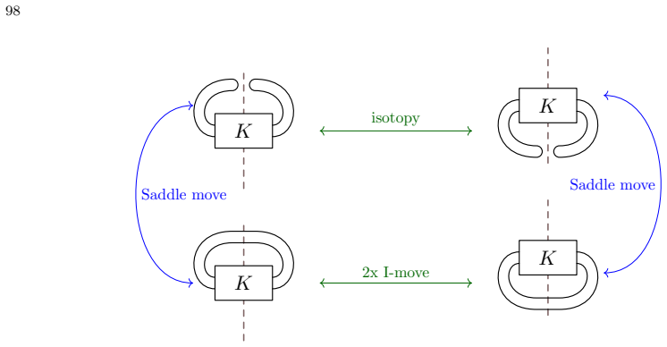
A set of 39 equivariant movie moves connects any two movie presentations of equivariantly isotopic cobordisms between involutive links.

A machine-rendered reading of the paper's core claim, the machinery that carries it, and where it could break.

The paper constructs an equivariant version of the Carter-Saito movie-move calculus for links that remain unchanged under 180-degree rotation in three-space. It proves that a concrete list of 39 local changes is sufficient to transform one movie diagram into another whenever the underlying cobordisms are related by an equivariant isotopy. The argument rests on a complete classification of codimension-two singularities that appear in equivariant projections together with an adaptation of embedded Morse theory to the rotational symmetry. This supplies a combinatorial toolkit for comparing and simplifying diagrams of surfaces that connect rotationally symmetric links.

Core claim

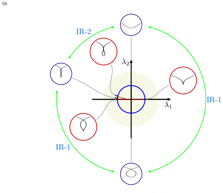
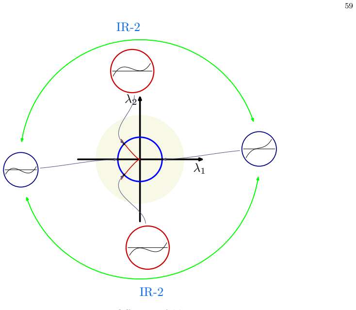
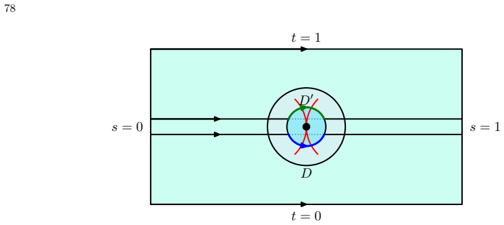
The authors prove that any two movie presentations of a pair of equivariantly isotopic cobordisms between involutive links can be related by a finite sequence drawn from a list of 39 specific equivariant movie moves. Along the way they give a singularity-theoretic proof of the equivariant Reidemeister theorem and examine the loops that arise from closed sequences of such moves. The proof proceeds by enumerating all codimension-two singularities of equivariant maps from the circle to the plane and by applying embedded equivariant Morse theory to control the changes that occur between regular levels.

What carries the argument

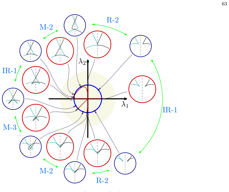
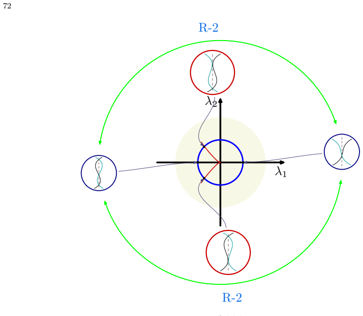
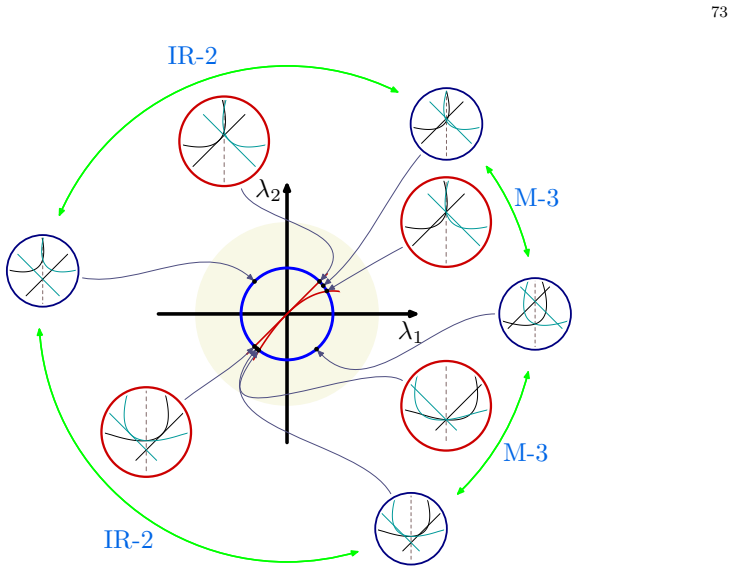
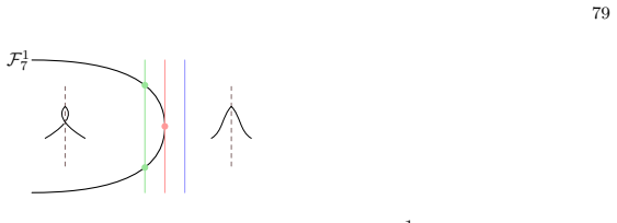
The 39 equivariant movie moves obtained from the classification of codimension-two singularities of equivariant maps S^1 to R^2.

Load-bearing premise

The classification of all codimension-two singularities of equivariant maps from the circle to the plane is exhaustive and embedded equivariant Morse theory introduces no further obstructions beyond those captured by the listed moves.

What would settle it

An explicit pair of movie diagrams representing equivariantly isotopic cobordisms that cannot be connected by the 39 moves, or an equivariant projection exhibiting a codimension-two singularity outside the enumerated types.
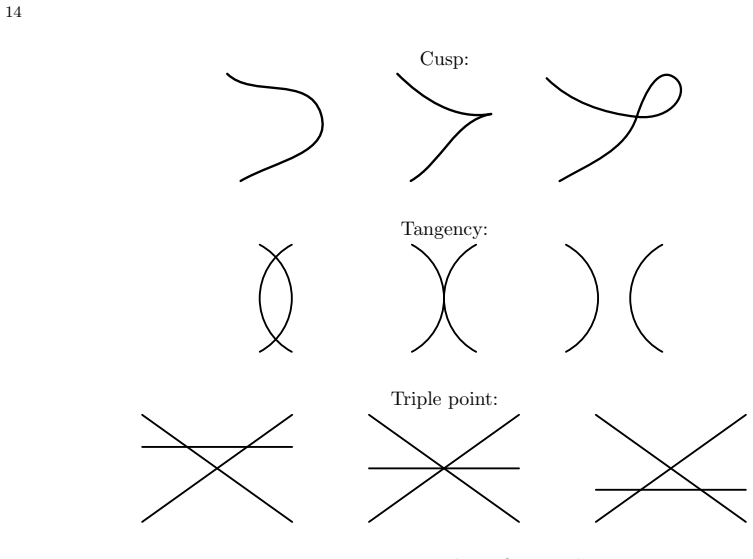
Figures

Figures reproduced from arXiv: 2604.26369 by Abhishek Mallick, Irving Dai, Maciej Borodzik, Matthew Stoffregen.

Figure 2.1
Figure 2.1. Figure 2.1: Perestroikas of critical points. A formal summary of this argument is given below: Corollary 2.21. Any two diagrams of the same knot can be connected by a sequence of isotopies and finitely many Reidemeister moves. Sketch of proof. A path ϕes : S → R 3 , s ∈ [0, 1] induces a path ϕs : S → R 2 via ϕs = π ◦ ϕes. We perturb ϕs to a regular path ϕs,n in such a way that ϕs,n agrees with ϕs for s = 0, 1. The p… view at source ↗
Figure 5.1
Figure 5.1. Figure 5.1: Top: a central tangency and an oblique tangency. Bottom: a perpendicular tangency and a fixed-point tangency. • Let ϕ ∈ O(t1, σt1) Z2 . We say ϕ is an on-axis perpendicular tangency if it satisfies Definition 5.27 at {t1, σt1} and ϕ ′ (t1) is horizontal. • Let ϕ ∈ O(t1, σt1, t2, σt2) Z2 . We say ϕ is an on-axis oblique tangency if it satisfies Definition 5.27 at either {t1, t2} or {t1, σt2} and ϕ(t1) ∈ L… view at source ↗
Figure 6.1
Figure 6.1. Figure 6.1: Top: bifurcation of an outer cusp. The middle picture shows the cusp singularity. Middle: bifurcation diagrams of an outer tangency. Bottom: bifurcation diagrams of an outer triple point. 6.1.3. Off-axis triple points. Define F 1 3 to be the space of ordinary triple points. Note that this comes from an ordinary strikethrough of the ordinary double point and hence has codi￾mension 1. Any extra tangency be… view at source ↗
Figure 6.2
Figure 6.2. Figure 6.2: Top: Bifurcation of central tangency. Middle: Bifurcation of perpendicularity tangency. Bottom: Bifurcaton of central double point. . 6.2.3. On-axis double point. Define F 1 6 to be the space of on-axis double points with no coincidences or strikethroughs, satisfying the additional condition that there are no tangencies between the four branches and that none of them are parallel or perpendicular to L. M… view at source ↗
Figure 6.3
Figure 6.3. Figure 6.3: Top: Bifurcation of a fixed point (2, 3) cusp. Bottom: Bifurca￾tion of a fixed double point. that for some t1 ∈ S− and t2 ∈ SZ2 , we have ϕ(t1) = ϕ(t2). To define F 1 8 , we require that none of {ϕ ′ (t1), τϕ′ (t1), ϕ′ (t2)} are parallel to each other (and that all of them are nonzero). Negating this condition adds an extra equation, so it is clear that Fe1 8 \ F1 8 consists of strata of codimension 2. A… view at source ↗
Figure 6.4
Figure 6.4. Figure 6.4: The equivariant Reidemeister moves. i = 1, 2. We assume r1 and r2 are sufficiently small so that they intersect K in small arc. Let κ be any smooth function which is zero inside C1 and π outside of C2. For s ∈ [0, 1], let ϕes : S 1 → R 3 by ϕes(u) = Rsκ(ϕe(u)) ◦ ϕe(u), where Rw is the rotation of R 3 about the z-axis by angle w. Clearly, ϕes consists of taking a knot and rotating all of it, except for th… view at source ↗
Figure 6.5
Figure 6.5. Figure 6.5: Crossing the point at infinity. Top: the fixed branch crosses the infinity point. Bottom: a pair of branches crossing the infinity point view at source ↗
Figure 6.6
Figure 6.6. Figure 6.6: Left: The I-move. The shaded part is the remaining diagram, which is not changed by the move. Right: the S-move. • If ti ∈ SZ2 , then a fixed-point branch of ϕsi hits ∞. As s varies, this fixed point sweeps over ∞ as indicated in view at source ↗
Figure 7.1
Figure 7.1. Figure 7.1: Off-axis singularities. From left-to-right: a (2, 5)-cusp, 2-fold tangency, strikethrough of a (2, 3)-cusp, strikethrough of a 1-fold tangency, and quadruple point. • ordinary strikethrough of an off-axis (2, 3)-cusp; • ordinary strikethrough of an off-axis 1-fold tangency; • ordinary strikethrough of an off-axis ordinary triple point (resulting in an off-axis quadruple point), called the X9 singularity.… view at source ↗
Figure 7.2
Figure 7.2. Figure 7.2: Off-axis (2, 5)-cusp. 7.2.2. 2-fold tangency. By Lemma 5.35, a 2-fold tangency has normal form with two branches y = 0 and (x = t, y = t 3 ) and versal deformation which perturbs the second branch to (x = t, y = t 3 + λ1t + λ2). There are no cusps or triple points regardless of λ1, λ2. A 1-fold tangency will occur if y(t) has a double root, which occurs along the locus {4λ 3 1 = −27λ 2 2 } and leads to a… view at source ↗
Figure 7.3
Figure 7.3. Figure 7.3: Off-axis 2-fold tangency. λ1 λ2 IR-3 IR-2 IR-1 IR-2 IR-1 view at source ↗
Figure 7.4
Figure 7.4. Figure 7.4: Strikethrough of an off-axis (2, 3)-cusp view at source ↗
Figure 7.5
Figure 7.5. Figure 7.5: Strikethrough of an off-axis 1-fold tangency. these. This occurs along the locus {λ2 = ± √ −λ1, λ1 ≤ 0}, leading to an (IR-3) move. The diagram is given in view at source ↗
Figure 7.6
Figure 7.6. Figure 7.6: Off-axis quadruple point view at source ↗
Figure 7.7
Figure 7.7. Figure 7.7: On-axis and fixed-point cusps. From left-to-right: an oblique (2, 3)-cusp, fixed-point (2, 5)-cusp, and fixed-point (3, 4)-cusp. the loci {λ1 = 0}, {λ2 = 0}, {λ1 = λ2}, and {λ1 = −λ2}, leading to (IR-3) moves. The diagram is given in view at source ↗
Figure 7.8
Figure 7.8. Figure 7.8: Oblique (2,3)-cusp. λ1 = −0.02 λ1 = −0.01 λ1 = −0.005 λ1 = 0 λ1 = 0.01 view at source ↗
Figure 7.10
Figure 7.10. Figure 7.10: Fixed-point (2, 5)-cusp. To determine the occurrence of other singularities, we first understand how our branch intersects itself. Setting p = t + t ′ , q = tt′ gives the identities t 2 − t ′2 = (t − t ′ )p, t3 − t ′3 = (t − t ′ )(p 2 − q), t4 − t ′4 = (t − t ′ )(p 3 − 2pq). Substituting these into x(t) = x(t ′ ) and y(t) = y(t ′ ) yields (7.6) p 2 − q + λ1 = 0, p3 − 2pq + λ2p = 0. Factor the second equ… view at source ↗
Figure 7.11
Figure 7.11. Figure 7.11: Fixed-point (3, 4)-cusp. the first class of solution to (7.6) gives λ1 = 0, while combining p 2 = 4q with the second gives 2λ1 = 3λ2. Both of these are subsumed by our casework for cusps. However, there is one more possibility for a tangency. This occurs when the two classes of solutions in p and q collide; i.e., when λ2 −2λ1 = 0. Note that in this case we require λ1 ≤ 0, so that p = t + t ′ = 0 and q =… view at source ↗
Figure 7.12
Figure 7.12. Figure 7.12: On-axis and fixed-point strikethroughs. From left-to-right: strikethrough of a line tangency, strikethrough of a perpendicular tangency, strikethrough of an on-axis double point, strikethrough of a fixed-point cusp, and strikethrough of a fixed double point. λ1 λ2 R-2 M-3 M-3 R-2 view at source ↗
Figure 7.13
Figure 7.13. Figure 7.13: Strikethrough of a 1-fold line tangency. is given by E1 = {x = t 2 + λ1, y = t}, E2 = {y = x − λ2}, with symmetric branches E3 = τ (E1) = {x = −t 2 − λ1, y = t}, E4 = τ (E2) = {y = −x − λ2}. For small values of λ1, λ2, the only tangency is between E1 and E3. This is a line tangency, which persists along the locus {λ1 = 0}. If λ1 > 0, then E1 and E3 are disjoint, leading to a regular diagram. For λ1 ≤ 0,… view at source ↗
Figure 7.14
Figure 7.14. Figure 7.14: Strikethrough of a 2-fold perpendicular tangency. 7.4.2. Strikethrough of a 2-fold perpendicular tangency. This has normal form (x = t, y = t 3 ) and y = ax for some a ̸= 0. Up to reparameterizing, we can assume a = 1. A versal deformation is given by E1 = {x = t, y = t 3 + λ1t}, E2 = {y = x + λ2}, with symmetric branches E3 = τ (E1) = {x = −t, y = t 3 + λ1t}, E4 = τ (E2) = {y = −x + λ2}. For small valu… view at source ↗
Figure 7.15
Figure 7.15. Figure 7.15: Strikethrough of a central double point. The deformation parameters are λ1, λ2, and a3. However, as in Section 7.2.5, we can freeze the a3 variable, leading to a3 being constant. For explicitness, we take a3 = 0.4, so that the slopes of the three lines are approximately ±22.5 ◦ , ±45◦ , and ±67.5 ◦ . No matter what the parameters λ1, λ2 are, each pair of lines intersects transversely. The lines E1, E2, … view at source ↗
Figure 7.16
Figure 7.16. Figure 7.16: Strikethrough of a fixed-point (2, 3)-cusp. λ1 = 0.005 λ1 = 0 λ1 = −0.005 λ1 = −0.01 λ1 = −0.015 view at source ↗
Figure 7.17
Figure 7.17. Figure 7.17: Close-up picture for λ1 ∼ 0 and λ2 ∼ 0.2. we have an on-axis double point. This occurs along the locus {λ1 = λ2, λ2 ≥ 0}, leading to an (M-3) move. As for tangencies, E2 is transverse to E3, so we consider tangencies between E1 and E2. For this, we find intersections between E1 and E2 and solve for a double root. Substituting the defining equations for E1 into that of E2, we must find when t 3 − t 2 − λ… view at source ↗
Figure 7.18
Figure 7.18. Figure 7.18: Close-up picture for λ1 ∼ 0 and λ2 ∼ −0.2. 7.4.5. Strikethrough of a fixed double point. We assume the branches involved in the fixed double point are y = 0 and y = a1x, along with its symmetric copy y = −a1x. Let the strikethrough line be y = a2x. By rescaling x and y, we can choose a1, as long as a1 ̸= 0 and a1 ̸= a2, but we cannot fix a2. For explicitness, we suppose a1 = 1/2. A versal deformation is… view at source ↗
Figure 7.19
Figure 7.19. Figure 7.19: Strikethrough of a fixed double point view at source ↗
Figure 7.20
Figure 7.20. Figure 7.20: On-axis and fixed-point tangencies. From left-to-right: 2-fold line tangency, 4-fold perpendicular tangency, 1-fold oblique tangency, fixed￾point (1, 2)-fold tangency, and a fixed-point branch intersecting a 1-fold line tangency. that our branch intersects its symmetric copy only at points on the x-axis. Hence tangencies occur when y(t) and y ′ (t) have a common root. This leads to t 4 + λ1t 2 + λ2 = 0 … view at source ↗
Figure 7.21
Figure 7.21. Figure 7.21: 2-fold line tangency. λ1 λ2 IR-2 M-2 M-2 view at source ↗
Figure 7.22
Figure 7.22. Figure 7.22: 4-fold perpendicular tangency view at source ↗
Figure 7.23
Figure 7.23. Figure 7.23: 1-fold oblique tangency. with symmetric branches E3 = τ (E1) = {u = λ1}, E4 = τ (E2) = {u = v 2 + λ2}. There are clearly no cusps. For λ1 = λ2, the tangency between E1 and E2 persists, and for small values of λ1, λ2 there are no other tangencies. Hence we obtain an off-axis tangency along the locus {λ1 = λ2}, leading to an (IR-2) move. To understand further singularities, we first determine the intersec… view at source ↗
Figure 7.24
Figure 7.24. Figure 7.24: Fixed-point (1, 2)-tangency. λ2 = −0.02 λ2 = −0.012 λ2 = −0.005 λ2 = 0 λ2 = 0.015 view at source ↗
Figure 7.25
Figure 7.25. Figure 7.25: Close-up picture for λ1 ∼ 0.2 and λ2 ∼ 0. λ2 = 0.015 λ2 = 0 λ2 = −0.005 λ2 = −0.013 λ2 = −0.02 view at source ↗
Figure 7.26
Figure 7.26. Figure 7.26: Close-up picture for λ1 ∼ −0.2 and λ2 ∼ 0. Reidemeister moves. We claim that one can pass from one sequence of Reidemeister moves to the other via a sequence of the following operations: (C-1) Replacing the order of two planar Reidemeister moves appearing in different places. (C-2) Introducing a birth or death of a pair of mutually inverse planar Reidemeister moves; that is, a planar Reidemeister move f… view at source ↗
Figure 7.27
Figure 7.27. Figure 7.27: Intersection of a fixed-point branch with 1-fold line tangency. Proof. We first observe that the two paths ϕs,0 and ϕs,1 are obviously path-homotopic via the linear homotopy ϕs,t = (1 − t)ϕs,0 + tϕs,1 defined for s, t ∈ [0, 1]. Note that each ϕs,t is indeed an equivariant map from S into R 2 . We aim to perturb ϕs,t to be generic, but first we have to define the space F 2 . Let F 2 0 be the subset of ma… view at source ↗
Figure 7
Figure 7. Figure 7: that goes along the upper arc of view at source ↗
Figure 7.28
Figure 7.28. Figure 7.28: Proof of Theorem 7.7. The two paths of Reidemeister moves differ by replacing a part of ∂D′ with the complement going in the opposite direction. The two arcs passing through the center of the disk represent the discriminant locus. If the singularity is not simple, then a few more details are needed. In each non-simple case instead of specifying a versal deformation, we produced a family transverse to th… view at source ↗
Figure 7.29
Figure 7.29. Figure 7.29: A schematic of a path which is non-transverse to F 1 . The three vertical lines represent three paths in the function space. The one to the right does not intersect the F 1 7 -stratum. The middle one is tangent to the stratum. Moving the path to the left creates two transverse intersection points with the F 1 7 -stratum. Each of the two points corresponds to an (R-1) move. locus corresponds to doing the… view at source ↗
Figure 8.1
Figure 8.1. Figure 8.1: Critical points outside the symmetry axis birth death saddle view at source ↗
Figure 8.2
Figure 8.2. Figure 8.2: Critical points on the symmetry axis • Critical points outside M ∩ Ω τ . The local form is ±x 2 1 ± x 2 2 + w1. Depending on signs we have: – A pair of births with the local form x 2 1 + x 2 2 + w1; – A pair of saddle points with the local form −x 2 1 + x 2 2 + w1; – A pair of deaths with the local form −x 2 1 − x 2 2 + w1. • A critical point in M ∩ Ω τ has local form ±x 2 1 ± y 2 1 + w1. Depending on si… view at source ↗
Figure 8.3
Figure 8.3. Figure 8.3: In these coordinates, we can specify what we mean by a good projection. Here, by a projection, we mean a smooth equivariant fibration R 3 → R 2 with fibers R. In general, we will consider projections that are C 1 -small perturbations of linear projections. Definition 8.27. A projection π : Rt0 → R 2 is good if it satisfies the following properties. (P-1) If u0 ∈/ Mτ , then π(u0) ∈ L/ ; (P-2) The vectors … view at source ↗
Figure 8.3
Figure 8.3. Figure 8.3: The surface M (left) and its intersection with the singular level set (right). We omit the v1–coordinate on both pictures. We defer the proof that good projections exist until Subsection 8.4.4. 8.4.2. Local compression of M and equivariant Morse moves. Suppose u0 is a critical point of F|M, but not of F itself. Let π be a good projection. Define the surface M′ ⊂ R 2 × [t0 − ε, t0 + ε] = {(π(u), F(u)): u … view at source ↗
Figure 8.4
Figure 8.4. Figure 8.4: Failure to regularity. Each linear equivariant projection takes the circle to the interval containing the image of the center. U ∩ Rt0 and equal to 1 on a smaller neighborhood of (0, 0, 0) ∈ Rt0 . Consider an equivariant map Ξ: Rt0 × R 2 → R 2 × R 2 by Ξ(x1, y1, v1, σ, ϕ) = (cos(ϕ)x1 + sin(ϕ)v1, y1 + σ(1 − θ)x 2 1 , σ, ϕ). If for some ϕ, σ, the preimage Ξ−1 (0, 0, σ, ϕ) does not contain any point of X ou… view at source ↗
Figure 9.1
Figure 9.1. Figure 9.1: R-1 move at infinity induces a loop. We have R-1 move, then a sequence of I- and S-moves, the inverse of R-1 move and the I-move again. K K K K K view at source ↗
Figure 9.2
Figure 9.2. Figure 9.2: R-2 move at infinity induces a loop. We have R-2 move, then a sequence of two S-moves, the inverse of R-2 move and then an isotopy. K K K K K view at source ↗
Figure 9.3
Figure 9.3. Figure 9.3: The loop of M-1 moves around infinity. We have M-1 move, then a sequence of I- and S-moves, the inverse of M-1 move and then a sequence of I- and S- moves. K K K K K view at source ↗
Figure 9.4
Figure 9.4. Figure 9.4: The loop of M-2 moves around infinity. The M-2 move is followed by S-moves and Reidemeister moves, then M-2 is undone and the S-move is applied. 9.4. Case (ML-2). The Morse point at infinity. This is the situation where there is a point x ∈ Σ that is mapped to ∞ × {t∞ i (s)} and it is a critical point of Hs at the same time. A dimension counting argument does not prohibit this situation. However, again b… view at source ↗
Figure 9.5
Figure 9.5. Figure 9.5: The loop of M-3 moves around infinity. The M-3 move is done. Then follows a sequence of S-moves and Reidemeister moves, then M-3 is undone. Finally, a sequence of S-moves and Reidemeister moves is done. K K K K Morse move Morse move I-move I-move view at source ↗
Figure 9.6
Figure 9.6. Figure 9.6: A loop of birth/death at infinity. The discussion in Subsection 8.4 implies that the diagram of the link obtained via π ι changes as in view at source ↗
Figure 9.7
Figure 9.7. Figure 9.7: The loop of saddle at infinity view at source ↗
Figure 9.8
Figure 9.8. Figure 9.8: Singular level set for a pair of saddles on-axis. The blue and red lines indicate singular level sets for u0 and u1. enough that neither axis is parallel to or perpendicular to the symmetry axis L), the non￾generic leads to a codimension 2 behavior. With these choices, the diagram above the level set looks locally as in the middle picture in the bottom row of view at source ↗
Figure 9.9
Figure 9.9. Figure 9.9: A loop for an orbit of handles hitting the symmetry axis. The Morse label indicates birth or death depending on the direction. The diagram on the top is an empty diagram (other components of the link might be present, but do not interfere. R-2 IR-2 IR-2 R-2 isotopy isotopy saddle singular saddles saddle view at source ↗
Figure 9.10
Figure 9.10. Figure 9.10: A loop for an orbit of handles on the symmetry axis. Saddle. [Gil82]. Recall that the changes of the link diagram are given by images of level sets of Hs under the map π ◦ Φs. The non-equivariant case. Dimension counting arguments indicate that π ◦ Φs must have the mildest possible (codimension 1) singularity as a map from R 2 to R 2 . Low-codimension singularities of such maps have been classified, and… view at source ↗
Figure 9.11
Figure 9.11. Figure 9.11: Case (ML-4). The dotted vertical line is the fold axis. The images of level sets of Hs under the fold map are circles with one double point view at source ↗
Figure 9.12
Figure 9.12. Figure 9.12: Case (ML-4), continued. If the critical point is moved away from the fold line, the level sets for small parameter are mapped into simple closed curves. A crossing occurs when the level sets cross the fold line. Instead, we assume that Hs(u1, u2) = B(u1, u2) + . . . , where B is a quadratic part and the dots denote higher order terms (of order 3 and more). The quadratic part is nondegenerate. Suppose B … view at source ↗
Figure 9.13
Figure 9.13. Figure 9.13: Case (ML-4), saddle point. The dotted vertical line is the fold axis. One set of hyperbolas (corresponding to the level sets of Hs below or above the critical point) are mapped bijectively by the fold map. The other set (corresponding to the opposite level sets) acquire a double point after the fold map. IR-1 IR-1 IR-1 Morse Morse view at source ↗
Figure 9.14
Figure 9.14. Figure 9.14: Twisted birth and death off-axis. The diagram is mirrored on the other side of the axis. In the middle diagrams, the smaller loop is done/undone by an IR-1 move. The equivariant case off-axis. This case is analogous to the non-equivariant case: the same movie is performed on both sides of the axis. That is, we have the following two off-axis movies from case (ML-4). We refer to them as singular Morse ha… view at source ↗
Figure 9.15
Figure 9.15. Figure 9.15: Twisted saddle off-axis. The diagram is mirrored on the other side of the axis. In the row, the R-1 moves are performed. IR-1 Saddle IR-1 Saddle view at source ↗
Figure 9.16
Figure 9.16. Figure 9.16: An actual movie move associated to the loop in view at source ↗
Figure 9.17
Figure 9.17. Figure 9.17: Twisted birth/death on-axis. R-1 R-1 view at source ↗
Figure 9.18
Figure 9.18. Figure 9.18: Twisted saddle on-axis. The arrows indicate the Morse moves (saddles). The row consists of Reidemeister moves. case: if the critical point is moved above the line {y1 = 0}, small ellipses (level sets of Hs) are disjoint from {y1 = 0}, and so, they are mapped curves with no self-intersections. Once they touch {y1 = 0}, they acquire a cusp and higher values of Hs lead to the circle with self-intersection.… view at source ↗
Figure 9.19
Figure 9.19. Figure 9.19: Birth/death over a point off-axis. IR-2 IR-2 view at source ↗
Figure 9.20
Figure 9.20. Figure 9.20: Saddle over a point off-axis. The arrows indicate the Morse move. Notice that neither the birth nor the saddle can possibly occur at the image of S Z2 . Indeed, this would mean that two fixed point of the τ action (the critical point and the point of S Z2 ) are mapped to the same point on L. This would imply that they are the same point, violating the assumption that ϕs is an embedding. The deformation … view at source ↗
Figure 9.21
Figure 9.21. Figure 9.21: Birth/death over a point on-axis M-1 M-1 view at source ↗
Figure 9.22
Figure 9.22. Figure 9.22: Saddle over a point on-axis view at source ↗
Figure 9.23
Figure 9.23. Figure 9.23: Birth and saddle off-axis can cancel. (NM-1) birth+saddle off-axis, see view at source ↗
Figure 9.24
Figure 9.24. Figure 9.24: Birth and saddle on-axis can cancel view at source ↗
Figure 9.25
Figure 9.25. Figure 9.25: Collision of critical points. A birth on the axis and a pair of saddles off-axis are equivalent to a saddle on-axis view at source ↗
Figure 9.26
Figure 9.26. Figure 9.26: Collision of critical points. A birth off the axis and a saddle on the axis can be traded for a birth on the axis. It might happen, for finitely many pairs (s0, t0) that ϕs0,t0 ∈ F2 , in which case the whole family is an unfolding of a codimension 2 Reidemeister singularity. This leads to one of the 18 loop (L-1)–(L-18) displayed in view at source ↗
read the original abstract

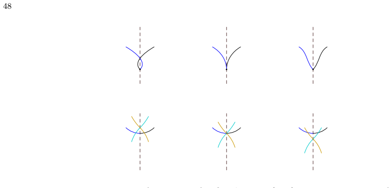
An involutive link is a link which is invariant under the standard rotation by 180 degrees in $S^3$. We establish an equivariant analogue of the work of Carter and Saito aimed at studying equivariant cobordisms between involutive links. This gives a set of $39$ equivariant movie moves that suffice to go between any two movie presentations of a pair of equivariantly isotopic cobordisms. Along the way, we give a singularity-theoretic proof of the equivariant Reidemeister theorem and study loops of equivariant Reidemeister moves. Our approach proceeds by analyzing codimension $2$ singularities of equivariant maps from $S^1$ to $\mathbb{R}^2$, as well as utilizing embedded equivariant Morse theory.

Editorial analysis

A structured set of objections, weighed in public.

Desk editor's note, referee report, simulated authors' rebuttal, and a circularity audit. Tearing a paper down is the easy half of reading it; the pith above is the substance, this is the friction.

Referee Report

2 major / 2 minor

Summary. The manuscript establishes an equivariant analogue of Carter-Saito movie moves for involutive links (links invariant under 180° rotation in S^3). It provides a singularity-theoretic proof of an equivariant Reidemeister theorem and derives a set of 39 equivariant movie moves that connect any two movie presentations of equivariantly isotopic cobordisms, via analysis of codimension-2 singularities of equivariant maps S^1 → R^2 together with embedded equivariant Morse theory.

Significance. If the classification of singularities is complete and the moves are exhaustive, the result supplies a concrete combinatorial framework for equivariant cobordisms, extending classical 3- and 4-dimensional knot theory to the involutive setting. This could enable systematic study of equivariant invariants and cobordism classes that are currently inaccessible by non-equivariant methods.

major comments (2)
  1. [Abstract and singularity-analysis section] The central claim that exactly 39 moves suffice rests on the completeness of the codimension-2 singularity classification for equivariant maps S^1 → R^2 under the fixed 180° rotation action. The abstract states that the authors analyze these singularities, but without an explicit enumeration of all local models, a proof that no additional singularities arise, and a verification that the listed moves generate all relations, the sufficiency of the 39 moves cannot be confirmed. This is load-bearing for both the Reidemeister theorem and the movie-move theorem.
  2. [Section on embedded equivariant Morse theory] The extension from the equivariant Reidemeister theorem to 1-parameter families (movie moves) assumes that embedded equivariant Morse theory introduces no extra obstructions beyond the enumerated singularities. The manuscript should contain a precise statement of the equivariant Morse lemma used and a check that the listed moves capture all possible births/deaths and handle crossings under the involution.
minor comments (2)
  1. [Abstract] The abstract introduces the 39 moves without indicating how many arise from Reidemeister-type moves versus Morse-type moves; a short breakdown would improve readability.
  2. [Introduction] Notation for the involution and the equivariant maps should be fixed early and used consistently when describing the local models.

Simulated Author's Rebuttal

2 responses · 0 unresolved

We thank the referee for their detailed and constructive report. The two major comments identify areas where the exposition can be strengthened to make the completeness arguments more transparent. We address each point below and outline the revisions we will incorporate.

read point-by-point responses
  1. Referee: [Abstract and singularity-analysis section] The central claim that exactly 39 moves suffice rests on the completeness of the codimension-2 singularity classification for equivariant maps S^1 → R^2 under the fixed 180° rotation action. The abstract states that the authors analyze these singularities, but without an explicit enumeration of all local models, a proof that no additional singularities arise, and a verification that the listed moves generate all relations, the sufficiency of the 39 moves cannot be confirmed. This is load-bearing for both the Reidemeister theorem and the movie-move theorem.

    Authors: We agree that explicitness is essential for the load-bearing claim. Section 3 of the manuscript classifies the codimension-2 singularities of equivariant maps S^1 → R^2 by stratifying according to orbit type (fixed-point loci and free orbits) and enumerates the admissible local models that arise in generic 1-parameter families. The 39 movie moves are derived directly from these models, and the text argues that they exhaust the relations by showing that all codimension-2 events are captured by the listed configurations. To make the argument fully transparent, we will add a new subsection that (i) tabulates every local model with its normal form and symmetry type, (ii) sketches the jet-space argument showing no further singularities appear under the Z/2-action, and (iii) cross-references each move to its originating singularity. These additions will be placed immediately after the current classification and will not alter the count of 39 moves. revision: partial

  2. Referee: [Section on embedded equivariant Morse theory] The extension from the equivariant Reidemeister theorem to 1-parameter families (movie moves) assumes that embedded equivariant Morse theory introduces no extra obstructions beyond the enumerated singularities. The manuscript should contain a precise statement of the equivariant Morse lemma used and a check that the listed moves capture all possible births/deaths and handle crossings under the involution.

    Authors: We concur that a self-contained statement of the lemma will clarify the passage from Reidemeister moves to movie moves. The manuscript applies an embedded equivariant Morse lemma asserting that a generic equivariant height function on an involutive surface has only non-degenerate critical points that are either fixed by the involution or occur in symmetric pairs, with births, deaths, and handle attachments respecting the symmetry. These events are already shown to correspond to the codimension-1 singularities already enumerated in the singularity analysis. We will insert an explicit statement of this lemma (with a short proof sketch adapted from the non-equivariant case) at the beginning of the embedded Morse theory section and add a short paragraph verifying that every birth/death or handle-crossing configuration under the involution is realized by one of the 39 moves. No new moves are required. revision: yes

Circularity Check

0 steps flagged

No circularity; derivation proceeds from independent singularity classification

full rationale

The paper establishes the 39 equivariant movie moves by performing a direct classification of codimension-2 singularities for equivariant maps S^1 → R^2 and applying embedded equivariant Morse theory to 1-parameter families. This analysis is carried out within the present work (including a self-contained proof of the equivariant Reidemeister theorem) and does not reduce any claimed prediction or completeness statement to a fitted parameter, self-definition, or load-bearing self-citation. The central result therefore rests on an independent enumeration rather than on any of the enumerated circularity patterns.

Axiom & Free-Parameter Ledger

0 free parameters · 2 axioms · 0 invented entities

The work rests on standard background results in differential topology and singularity theory rather than introducing new free parameters or invented entities.

axioms (2)
  • standard math Standard properties of smooth manifolds, embeddings, and isotopies in dimensions 3 and 4
    Invoked throughout the definitions of involutive links, equivariant cobordisms, and movie presentations.
  • domain assumption Completeness of the classification of codimension-2 singularities for equivariant maps S^1 to R^2
    Central to the singularity-theoretic approach described in the abstract.

pith-pipeline@v0.9.0 · 5426 in / 1349 out tokens · 41708 ms · 2026-05-07T12:33:00.008178+00:00 · methodology

discussion (0)

Sign in with ORCID, Apple, or X to comment. Anyone can read and Pith papers without signing in.

Reference graph

Works this paper leans on

57 extracted references · 7 canonical work pages

  1. [1]

    auser Classics, Birkh\

    V. I. Arnold, S. M. Gusein-Zade, and A. N. Varchenko, Singularities of differentiable maps. V olume 1 , Modern Birkh\"auser Classics, Birkh\"auser/Springer, New York, 2012, Classification of critical points, caustics and wave fronts, Translated from the Russian by Ian Porteous based on a previous translation by Mark Reynolds, Reprint of the 1985 edition. 2896292

  2. [2]

    Manabu Akaho, Morse homology and manifolds with boundary, Commun. Contemp. Math. 9 (2007), no. 3, 301--334. 2336820

  3. [3]

    Manabu Akaho, Morse homology of manifolds with boundary revisited, preprint, arXiv:1408.1474

  4. [4]

    V. I. Arnold, Geometrical methods in the theory of ordinary differential equations, second ed., Grundlehren der mathematischen Wissenschaften [Fundamental Principles of Mathematical Sciences], vol. 250, Springer-Verlag, New York, 1988, Translated from the Russian by Joseph Sz\" u cs [J\' o zsef M. Sz u cs]. 947141

  5. [5]

    Soviet Math., vol

    , Plane curves, their invariants, perestroikas and classifications, Singularities and bifurcations, Adv. Soviet Math., vol. 21, Amer. Math. Soc., Providence, RI, 1994, With an appendix by F. Aicardi, pp. 33--91. 1310595

  6. [6]

    Maciej Borodzik and Weronika Buczyńska, Families of M orse functions for manifolds with boundary , preprint, arXiv 2507.15847

  7. [7]

    Keegan Boyle and Wenzhao Chen, Equivariant unknotting numbers of strongly invertible knots, 2025, preprint, arXiv 2412.09797

  8. [8]

    Maciej Borodzik, Irving Dai, Abhishek Mallick, and Matthew Stoffregen, Khovanov homology and equivariant surfaces, arXiv preprint arXiv:2507.13642 (2025)

  9. [9]

    Knot Theory Ramifications 19 (2010), no

    Christian Blanchet, An oriented model for K hovanov homology , J. Knot Theory Ramifications 19 (2010), no. 2, 291--312. 2647055

  10. [10]

    Dror Bar-Natan, Khovanov's homology for tangles and cobordisms, Geom. Topol. 9 (2005), 1443--1499. 2174270

  11. [11]

    Maciej Borodzik and Mark Powell, Embedded M orse T heory and R elative S plitting of C obordisms of M anifolds , J. Geom. Anal. 26 (2016), no. 1, 57--87. 3441503

  12. [12]

    Bredon, Introduction to compact transformation groups, Pure and Applied Mathematics, Vol

    Glen E. Bredon, Introduction to compact transformation groups, Pure and Applied Mathematics, Vol. 46, Academic Press, New York-London, 1972. 0413144

  13. [13]

    Maciej Borodzik and Henryk \.Zo adek, Complex algebraic plane curves via P oincar\'e- H opf formula. III . C odimension bounds , J. Math. Kyoto Univ. 48 (2008), no. 3, 529--570. 2511050

  14. [14]

    Jae Choon Cha and Ki Hyoung Ko, On equivariant slice knots, Proc. Amer. Math. Soc. 127 (1999), no. 7, 2175--2182. 1605928

  15. [15]

    David Clark, Scott Morrison, and Kevin Walker, Fixing the functoriality of K hovanov homology , Geom. Topol. 13 (2009), no. 3, 1499--1582. 2496052

  16. [16]

    Scott Carter, Joachim H

    J. Scott Carter, Joachim H. Rieger, and Masahico Saito, A combinatorial description of knotted surfaces and their isotopies, Adv. Math. 127 (1997), no. 1, 1--51. 1445361

  17. [17]

    Scott Carter and Masahico Saito, Reidemeister moves for surface isotopies and their interpretation as moves to movies, J

    J. Scott Carter and Masahico Saito, Reidemeister moves for surface isotopies and their interpretation as moves to movies, J. Knot Theory Ramifications 2 (1993), no. 3, 251--284. 1238875

  18. [18]

    J. M. S. David, Projection-generic curves, J. London Math. Soc. (2) 27 (1983), no. 3, 552--562. 697147

  19. [19]

    3, 1167--1236

    Irving Dai, Abhishek Mallick, and Matthew Stoffregen, Equivariant knots and knot F loer homology , Journal of Topology 16 (2023), no. 3, 1167--1236

  20. [20]

    Davis and Swatee Naik, Alexander polynomials of equivariant slice and ribbon knots in S^3 , Trans

    James F. Davis and Swatee Naik, Alexander polynomials of equivariant slice and ribbon knots in S^3 , Trans. Amer. Math. Soc. 358 (2006), no. 7, 2949--2964. 2216254

  21. [21]

    Alessio Di Prisa, The equivariant concordance group is not abelian, Bull. Lond. Math. Soc. 55 (2023), no. 1, 502--507. 4568356

  22. [22]

    , Equivariant algebraic concordance of strongly invertible knots, J. Topol. 17 (2024), no. 4, Paper No. e70006, 44. 4822933

  23. [23]

    Michael Ehrig, Daniel Tubbenhauer, and Paul Wedrich, Functoriality of colored link homologies, Proc. Lond. Math. Soc. (3) 117 (2018), no. 5, 996--1040. 3877770

  24. [24]

    Band 153, Springer-Verlag New York, Inc., New York, 1969

    Herbert Federer, Geometric measure theory, Die Grundlehren der mathematischen Wissenschaften, vol. Band 153, Springer-Verlag New York, Inc., New York, 1969. 257325

  25. [25]

    Thomas Fiedler and Vitaliy Kurlin, A 1-parameter approach to links in a solid torus, J. Math. Soc. Japan 62 (2010), no. 1, 167--211. 2648220

  26. [26]

    Golubitsky and V

    M. Golubitsky and V. Guillemin, Stable mappings and their singularities, Graduate Texts in Mathematics, Vol. 14, Springer-Verlag, New York-Heidelberg, 1973. 0341518

  27. [27]

    Giller, Towards a classical knot theory for surfaces in R 4 , Illinois J

    Cole A. Giller, Towards a classical knot theory for surfaces in R 4 , Illinois J. Math. 26 (1982), no. 4, 591--631. 674227

  28. [28]

    G. H. Hardy, Divergent series, \'Editions Jacques Gabay, Sceaux, 1992, With a preface by J. E. Littlewood and a note by L. S. Bosanquet, Reprint of the revised (1963) edition. 1188874

  29. [29]

    Kyle Hayden and Isaac Sundberg, Khovanov homology and exotic surfaces in the 4-ball, 2021, preprint, arXiv:2108.04810

  30. [30]

    Magnus Jacobsson, An invariant of link cobordisms from K hovanov homology , Algebr. Geom. Topol. 4 (2004), 1211--1251. 2113903

  31. [31]

    Mikhail Khovanov, A categorification of the J ones polynomial , Duke Math. J. 101 (2000), no. 3, 359--426. 1740682

  32. [32]

    , A functor-valued invariant of tangles, Algebr. Geom. Topol. 2 (2002), 665--741. 1928174

  33. [33]

    Robert Lipshitz and Sucharit Sarkar, Khovanov homology of strongly invertible knots and their quotients, Frontiers in geometry and topology, Proc. Sympos. Pure Math., vol. 109, Amer. Math. Soc., Providence, RI, [2024] 2024, pp. 157--182. 4772951

  34. [34]

    Andrew Lobb and Liam Watson, A refinement of K hovanov homology , Geom. Topol. 25 (2021), no. 4, 1861--1917. 4286365

  35. [35]

    4, e70001

    Abhishek Mallick, Knot F loer homology and surgery on equivariant knots , Journal of Topology 17 (2024), no. 4, e70001

  36. [36]

    Jean Martinet, D\'eploiements versels des applications diff\'erentiables et classification des applications stables, Singularit\'es d'applications diff\'erentiables ( S \'em., P lans-sur- B ex, 1975), Lecture Notes in Math., vol. Vol. 535, Springer, Berlin-New York, 1976, pp. 1--44. 649264

  37. [37]

    Morgan and Hyman Bass, The S mith conjecture , Pure Appl

    John W. Morgan and Hyman Bass, The S mith conjecture , Pure Appl. Math., vol. 112, Academic Press, Orlando, FL, 1984, pp. 3--6. 758460

  38. [38]

    Alice Merz, The A lexander and M arkov theorems for strongly involutive links , J. Lond. Math. Soc. (2) 111 (2025), no. 4, Paper No. e70156, 60. 4892887

  39. [39]

    Miller and Mark Powell, Strongly invertible knots, equivariant slice genera, and an equivariant algebraic concordance group, J

    Allison N. Miller and Mark Powell, Strongly invertible knots, equivariant slice genera, and an equivariant algebraic concordance group, J. Lond. Math. Soc. (2) 107 (2023), no. 6, 2025--2053. 4598178

  40. [40]

    Kunio Murasugi, On periodic knots, Comment. Math. Helv. 46 (1971), 162--174. 292060

  41. [41]

    Scott Morrison, Kevin Walker, and Paul Wedrich, Invariants of 4-manifolds from K hovanov- R ozansky link homology , Geom. Topol. 26 (2022), no. 8, 3367--3420. 4562565

  42. [42]

    Ciprian Manolescu, Kevin Walker, and Paul Wedrich, Skein lasagna modules and handle decompositions, Adv. Math. 425 (2023), Paper No. 109071, 40. 4589588

  43. [43]

    Swatee Naik, Periodicity, genera and A lexander polynomials of knots , Pacific J. Math. 166 (1994), no. 2, 357--371. 1313460

  44. [44]

    42, Polish Acad

    Dennis Roseman, Reidemeister-type moves for surfaces in four-dimensional space, Knot theory ( W arsaw, 1995), Banach Center Publ., vol. 42, Polish Acad. Sci. Inst. Math., Warsaw, 1998, pp. 347--380. 1634466

  45. [45]

    176--196

    Makoto Sakuma, On strongly invertible knots, Algebraic and topological theories ( K inosaki, 1984), Kinokuniya, Tokyo, 1986, pp. 176--196. 1102258

  46. [46]

    Taketo Sano, Involutive khovanov homology and equivariant knots, 2025

  47. [47]

    Math., vol

    Jan Stevens, On the classification of reducible curve singularities, Algebraic geometry and singularities ( L a R \'abida, 1991), Progr. Math., vol. 134, Birkh\"auser, Basel, 1996, pp. 383--407. 1395193

  48. [48]

    U ber I nvolutionen der 3 - S ph\

    Friedhelm Waldhausen, \" U ber I nvolutionen der 3 - S ph\" a re , Topology 8 (1969), 81--91. 236916

  49. [49]

    C. T. C. Wall, Equivariant jets, Math. Ann. 272 (1985), no. 1, 41--65. 794090

  50. [50]

    , Projection genericity of space curves, J. Topol. 1 (2008), no. 2, 362--390. 2399135

  51. [51]

    Wasserman, Equivariant differential topology, Topology 8 (1969), 127--150

    Arthur G. Wasserman, Equivariant differential topology, Topology 8 (1969), 127--150. 250324

  52. [52]

    Liam Watson, Khovanov homology and the symmetry group of a knot, Adv. Math. 313 (2017), 915--946. 3649241

  53. [53]

    Paul Wedrich, From link homology to topological quantum field theories, 2025, preprint, arXiv 2509.08478

  54. [54]

    4 (1937), 276--284

    Hassler Whitney, On regular closed curves in the plane, Compositio Math. 4 (1937), 276--284. 1556973

  55. [55]

    , Differentiable even functions, Duke Math. J. 10 (1943), 159--160. 7783

  56. [56]

    , On singularities of mappings of euclidean spaces. I . M appings of the plane into the plane , Ann. of Math. (2) 62 (1955), 374--410. 73980

  57. [57]

    Sarah Zampa, A bound on the equivariant unknotting number, 2025, preprint, 2512.17700