Recognition: unknown
Turbulence and its Potential Impact on Solar Chromospheric and Coronal Heating
Pith reviewed 2026-05-07 10:43 UTC · model grok-4.3
The pith
Turbulence from mixed polarity magnetic fields in the solar chromosphere supplies more energy than needed to heat both the chromosphere and corona.
A machine-rendered reading of the paper's core claim, the machinery that carries it, and where it could break.
Core claim
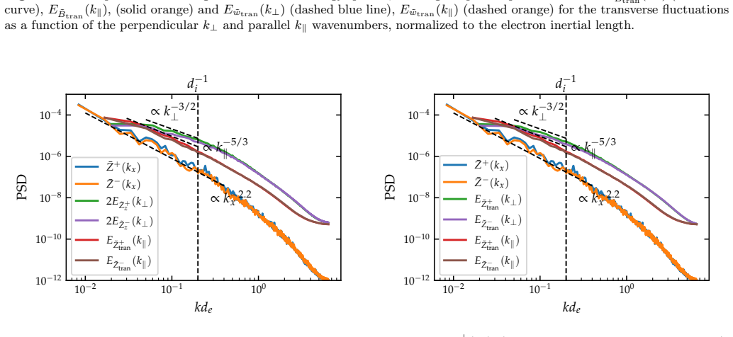
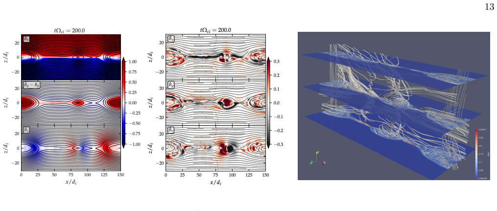
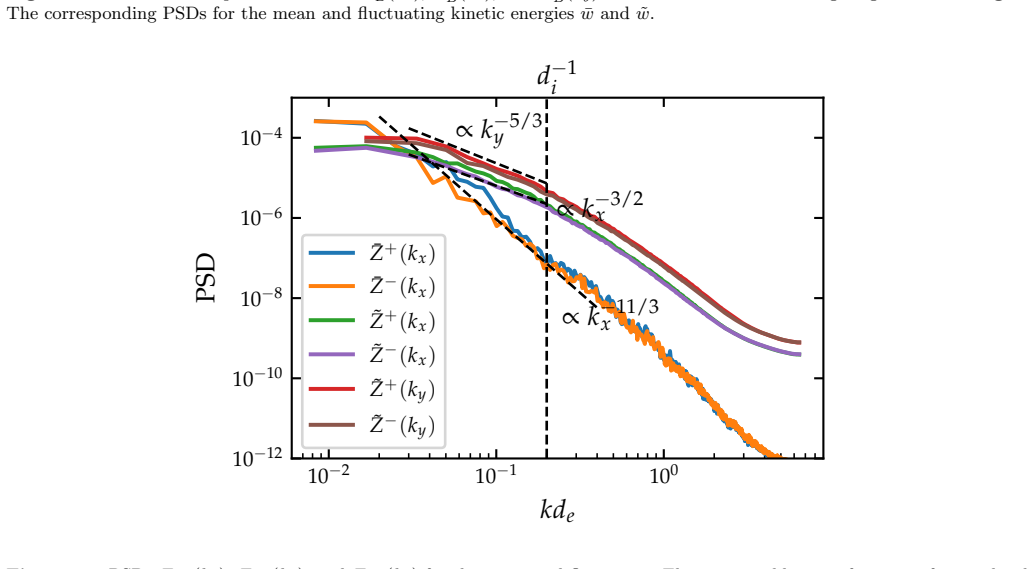
Simulations of emergent mixed polarity magnetic fields demonstrate a fast shift to a turbulent state with advected nonlinear structures and partial annihilation of the initial field. The transport model then predicts that the expected energy injection rates from this turbulence, both within the chromosphere and at the base of the corona, surpass the energy needed to sustain the observed temperatures in each layer.
What carries the argument
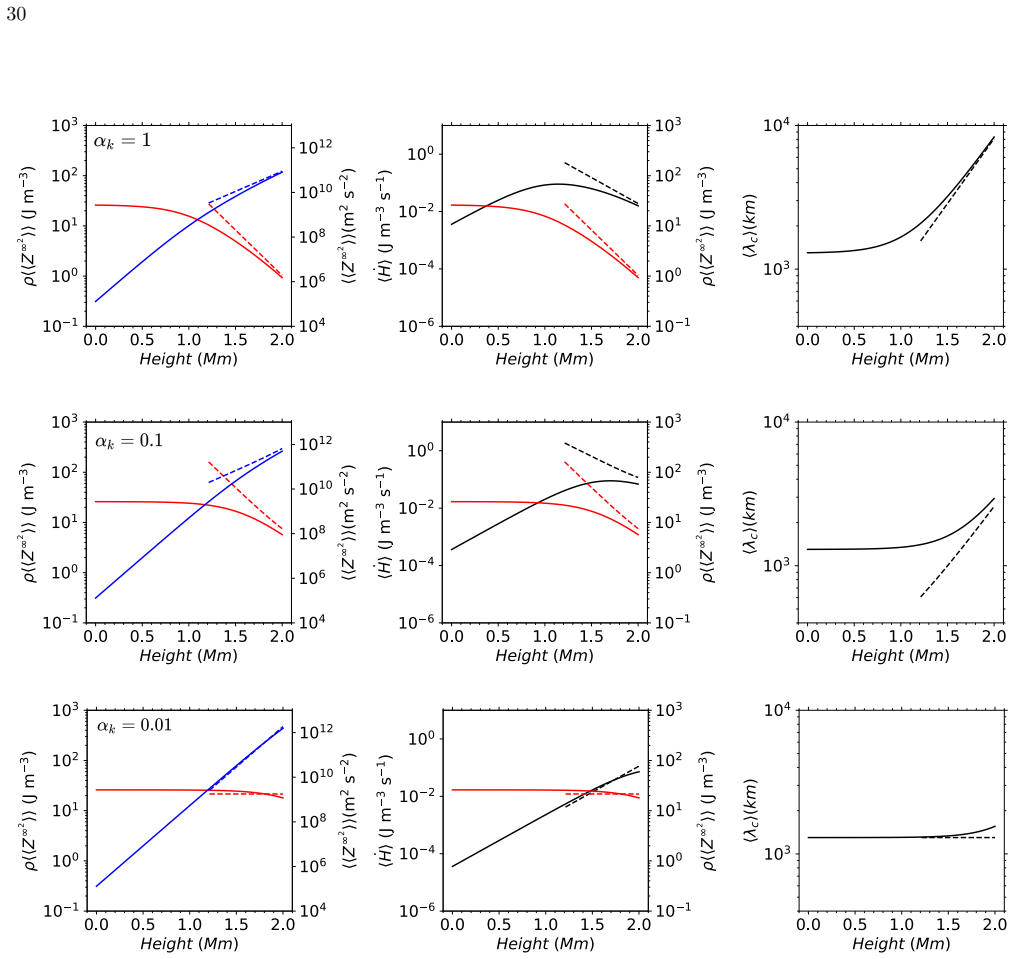
The transport model that advects and dissipates turbulence from randomly distributed energy-containing scale dynamical flows obeying log-normal statistics, yielding height-dependent expectations for total energy per unit volume, Elsasser specific energy, heating rate, and correlation length.
If this is right
- Turbulent energy injection exceeds the amount required to heat the chromosphere and the base of the corona.
- Spicules can receive gradual heating with increasing height through entrainment of magnetic carpet and photospheric turbulence.
- Turbulence remains anisotropic when the guide magnetic field is imbalanced and becomes more isotropic when the field is balanced.
- Energy reaches the low corona through a random patchwork of injection sites distributed across the transition region surface.
Where Pith is reading between the lines
- The same mechanism could operate in other stellar atmospheres that exhibit mixed polarity surface fields.
- Spectral observations of velocity or magnetic fluctuations in the chromosphere could directly test the predicted log-normal statistics of the energy-containing scales.
- Extending the model to include time-dependent or spatially clustered injection sites would allow comparison with localized heating events such as bright points.
Load-bearing premise
Energy-containing scale dynamical flows are randomly distributed throughout the chromosphere and obey log-normal statistics, with turbulence injected by a random patchwork of sites across the transition region surface.
What would settle it
In-situ or remote measurements showing energy injection rates from chromospheric turbulence that fall below the independently estimated heating requirements for the chromosphere or corona would falsify the central claim.
Figures


read the original abstract
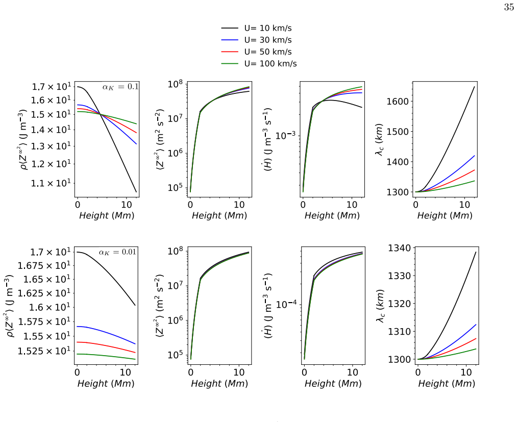
Low-frequency turbulence in the solar chromosphere remains poorly understood. We address 1) the sources of low-frequency turbulence that potentially heat the chromosphere, and 2) how turbulence is transported and dissipated throughout the chromosphere and lower corona. We use particle-in-cell simulations to investigate mixed polarity magnetic fields corresponding to emergent magnetic carpet field in coronal holes or quiet Sun regions for strong (imbalanced) and weak (balanced) guide magnetic fields. The initial mixed polarity magnetic field transitions rapidly to a turbulent state dominated by advected small-scale nonlinear structures, with a minority slab turbulence population and the emergent field is largely annihilated. Turbulence is anisotropic for imbalanced magnetic field and more isotropic for balanced cases. We develop a transport model for turbulence advected and dissipated throughout the chromosphere by randomly distributed energy-containing scale dynamical flows described by log-normal statistics. We compute the expectations for the total energy per unit volume <y>(h) J m^{-3}, the Elsasser specific energy <Z^{\infty 2}>(h) m^2 s^{-2}, the heating rate <\cdot{H}>(h) J m^{-3} s^{-1}, and the correlation length <{\lambda}>(h) km as functions of height h above the photosphere. Turbulent energy is injected into the low corona by a random "patchwork" of sites across the transition region surface. The expected energy injection rates <\cdot{S}> J m^{-2} s^{-1} for the chromosphere and at the base of the corona exceed the estimated energy requirements needed to heat both the chromosphere and corona. Similarly, we show that spicules can be heated gradually with increasing height by entrained magnetic carpet and photospheric turbulence.
Editorial analysis
A structured set of objections, weighed in public.
Referee Report
Summary. The manuscript reports particle-in-cell simulations of mixed-polarity magnetic fields representing the solar magnetic carpet, showing rapid transition to anisotropic (imbalanced guide field) or isotropic (balanced) turbulence with dominant advected nonlinear structures and largely annihilated emergent field. It then introduces a transport model in which energy-containing scale flows are assumed randomly distributed throughout the chromosphere and obey log-normal statistics; turbulence is injected via a random patchwork of sites at the transition region. Height-dependent expectations are computed for total energy density <y>(h), Elsasser energy <Z^∞²>(h), heating rate <H>(h), and correlation length <λ>(h). The central claim is that the resulting expected energy injection rates <S> exceed the energy requirements to heat the chromosphere and lower corona; spicules are also argued to be heated by entrained turbulence.
Significance. If the statistical assumptions hold and can be validated, the work would supply a concrete, observationally testable mechanism by which low-frequency turbulence from the magnetic carpet supplies the energy budget for chromospheric and coronal heating. The combination of PIC results on turbulence generation with an analytical transport model is a positive feature that could yield falsifiable predictions for height-dependent heating rates.
major comments (2)
- [Transport model and computation of expectations] The headline result that expected injection rates <S> exceed chromospheric and coronal heating requirements rests on the transport model whose inputs (log-normal parameters for energy-containing scale flows, random patchwork injection site density and strength) are free parameters not derived from or validated against the PIC simulation outputs. The simulations demonstrate turbulence and field annihilation but report no height-dependent statistical tests, correlation-length measurements, or distribution fits that would constrain these inputs.
- [Transport model] The expectations <y>(h), <Z^∞²>(h), <H>(h), and <λ>(h) are computed from an assumed log-normal distribution of randomly distributed dynamical flows, yet the manuscript provides no explicit derivation or justification linking this statistical form to the PIC results (which show rapid transition to turbulence but do not quantify the required height-dependent distributions or injection-site statistics).
minor comments (1)
- [Notation and definitions] Notation for expectations (e.g., <·S>, <H>(h)) should be defined explicitly at first use, with clear statements of which quantities are averaged over the random site distribution versus over the log-normal ensemble.
Simulated Author's Rebuttal
We thank the referee for their careful review and for highlighting the potential significance of combining PIC simulations of magnetic carpet turbulence with a statistical transport model. We address the major comments on the transport model below.
read point-by-point responses
-
Referee: [Transport model and computation of expectations] The headline result that expected injection rates <S> exceed chromospheric and coronal heating requirements rests on the transport model whose inputs (log-normal parameters for energy-containing scale flows, random patchwork injection site density and strength) are free parameters not derived from or validated against the PIC simulation outputs. The simulations demonstrate turbulence and field annihilation but report no height-dependent statistical tests, correlation-length measurements, or distribution fits that would constrain these inputs.
Authors: We agree that the specific parameter values in the transport model (log-normal moments, injection-site density and strength) are not obtained by direct statistical fitting to the PIC outputs. The PIC runs are designed to demonstrate the rapid onset of turbulence and field annihilation from mixed-polarity carpet fields, while the transport model is a separate, height-dependent statistical description. In the revised manuscript we will add an explicit subsection that (i) motivates the log-normal form from the multiplicative nature of the advected nonlinear structures seen in the simulations and (ii) presents a sensitivity analysis showing that the headline conclusion <S> exceeding heating requirements remains robust across a plausible range of parameters consistent with observed carpet properties. We will also clarify that full height-resolved validation would require larger-domain, stratified simulations that are beyond the scope of the present work. revision: partial
-
Referee: [Transport model] The expectations <y>(h), <Z^∞²>(h), <H>(h), and <λ>(h) are computed from an assumed log-normal distribution of randomly distributed dynamical flows, yet the manuscript provides no explicit derivation or justification linking this statistical form to the PIC results (which show rapid transition to turbulence but do not quantify the required height-dependent distributions or injection-site statistics).
Authors: The log-normal distribution is adopted because it is the natural outcome of multiplicative random processes that characterize the statistics of energy-containing eddies in developed turbulence; the PIC results show precisely such a rapid transition to a state dominated by advected nonlinear structures. We will revise the manuscript to include a concise derivation of why this statistical form is appropriate, referencing the observed dominance of advected structures and the annihilation of the emergent field in both the balanced and imbalanced cases. The height dependence itself is necessarily analytic because the PIC domain does not span the full chromospheric height range; we will state this limitation clearly and note that the model predictions can be tested against future observations of height-dependent correlation lengths and heating rates. revision: yes
Circularity Check
No significant circularity in derivation chain
full rationale
The paper uses PIC simulations to demonstrate rapid transition of mixed-polarity fields to anisotropic or isotropic turbulence with field annihilation. It then separately develops a transport model assuming randomly distributed energy-containing flows obeying log-normal statistics, with turbulence injected via a random patchwork of sites at the transition region. Expectations <y>(h), <Z^∞²>(h), <H>(h), <λ>(h), and <S> are computed from this model and compared to independent estimates of chromospheric/coronal heating requirements. No equation or step reduces by construction to its own inputs (no self-definition of the exceedance, no fitted parameter renamed as prediction, no load-bearing self-citation or uniqueness theorem). The statistical assumptions are explicit modeling choices whose justification is external to the derivation itself; the exceedance result is an output of the forward calculation rather than a tautology. The derivation chain is therefore self-contained.
Axiom & Free-Parameter Ledger
free parameters (2)
- log-normal parameters for energy-containing scale flows
- random patchwork injection site density and strength
axioms (2)
- domain assumption Turbulence generated by mixed-polarity magnetic fields can be treated as advected and dissipated by randomly distributed energy-containing flows
- domain assumption PIC simulation results for strong and weak guide fields provide representative initial conditions for the transport model
Reference graph
Works this paper leans on
-
[1]
2009, SoPh, 260, 43, doi: 10.1007/s11207-009-9433-7
Abramenko, V., Yurchyshyn, V., & Watanabe, H. 2009, SoPh, 260, 43, doi: 10.1007/s11207-009-9433-7
-
[2]
Abramenko, V. I., Zank, G. P., Dosch, A., et al. 2013, ApJ, 773, 167, doi: 10.1088/0004-637X/773/2/167
-
[3]
Adhikari, L., Zank, G. P., Telloni, D., et al. 2024a, ApJ, 966, 52, doi: 10.3847/1538-4357/ad3109
-
[4]
Adhikari, L., Zank, G. P., Telloni, D., & Zhao, L. L. 2022, ApJL, 937, L29, doi: 10.3847/2041-8213/ac91c6
-
[5]
Adhikari, L., Zank, G. P., Zhao, L., et al. 2024b, ApJ, 965, 94, doi: 10.3847/1538-4357/ad2fc4
-
[6]
Adhikari, L., Zank, G. P., & Zhao, L. L. 2020, ApJ, 901, 102, doi: 10.3847/1538-4357/abb132
-
[7]
2022, ApJL, 940, L13, doi: 10.3847/2041-8213/aca075
Benzi, R. 2022, ApJL, 940, L13, doi: 10.3847/2041-8213/aca075
-
[8]
Anderson, L. S., & Athay, R. G. 1989, ApJ, 346, 1010, doi: 10.1086/168083
-
[9]
Asgari-Targhi, M., & van Ballegooijen, A. A. 2012, ApJ, 746, 81, doi: 10.1088/0004-637X/746/1/81
-
[10]
Athay, R. G. 1966, ApJ, 146, 223, doi: 10.1086/148870
-
[11]
I., & McKenzie, J
Axford, W. I., & McKenzie, J. F. 1992, in Solar Wind Seven Colloquium, ed. E. Marsch & R. Schwenn, 1–5
1992
-
[12]
2025, ApJL, 980, L20, doi: 10.3847/2041-8213/ada363
Bailey, Z., Bandyopadhyay, R., Habbal, S., & Druckm¨ uller, M. 2025, ApJL, 980, L20, doi: 10.3847/2041-8213/ada363
-
[13]
Bale, S. D., Drake, J. F., McManus, M. D., et al. 2023, Nature, 618, 252, doi: 10.1038/s41586-023-05955-3
-
[14]
Bandyopadhyay, R., Matthaeus, W. H., McComas, D. J., et al. 2022, ApJL, 926, L1, doi: 10.3847/2041-8213/ac4a5c
-
[15]
Beckers, J. M. 1968, SoPh, 3, 367, doi: 10.1007/BF00171614
-
[16]
Beckers, J. M. 1972, ARA&A, 10, 73, doi: 10.1146/annurev.aa.10.090172.000445
-
[17]
E., Slater, G., Hurlburt, N., et al
Berger, T. E., Slater, G., Hurlburt, N., et al. 2010, ApJ, 716, 1288, doi: 10.1088/0004-637X/716/2/1288
-
[18]
J., Albright, B., Yin, L., Bergen, B., & Kwan, T
Bowers, K. J., Albright, B., Yin, L., Bergen, B., & Kwan, T. 2008, Physics of Plasmas (1994-present), 15, 055703
2008
-
[19]
Burlaga, L. F., & Szabo, A. 1999, SSRv, 87, 137, doi: 10.1023/A:1005186720589
-
[20]
Carlsson, M., De Pontieu, B., & Hansteen, V. H. 2019, ARA&A, 57, 189, doi: 10.1146/annurev-astro-081817-052044
-
[21]
A publicly available simulation of an enhanced network region of the Sun
Carlsson, M., Hansteen, V. H., Gudiksen, B. V., Leenaarts, J., & De Pontieu, B. 2016, A&A, 585, A4, doi: 10.1051/0004-6361/201527226
-
[22]
Carlsson, M., & Stein, R. F. 1997, ApJ, 481, 500, doi: 10.1086/304043
-
[23]
Chandran, B. D. G. 2021, Journal of Plasma Physics, 87, 905870304, doi: 10.1017/S0022377821000052
-
[24]
Chandran, B. D. G., Dennis, T. J., Quataert, E., & Bale, S. D. 2011, ApJ, 743, 197, doi: 10.1088/0004-637X/743/2/197
-
[25]
Chandran, B. D. G., & Hollweg, J. V. 2009, ApJ, 707, 1659, doi: 10.1088/0004-637X/707/2/1659
-
[26]
Chandran, B. D. G., & Perez, J. C. 2019, Journal of Plasma Physics, 85, 905850409, doi: 10.1017/S0022377819000540
-
[27]
Cranmer, S. R., & Molnar, M. E. 2023, ApJ, 955, 68, doi: 10.3847/1538-4357/acee6c 40
-
[28]
Cranmer, S. R., & van Ballegooijen, A. A. 2010, ApJ, 720, 824, doi: 10.1088/0004-637X/720/1/824
-
[29]
Cranmer, S. R., van Ballegooijen, A. A., & Edgar, R. J. 2007, ApJS, 171, 520, doi: 10.1086/518001
-
[30]
Cranmer, S. R., van Ballegooijen, A. A., & Woolsey, L. N. 2013, ApJ, 767, 125, doi: 10.1088/0004-637X/767/2/125 De Moortel, I., & Browning, P. 2015, Philosophical Transactions of the Royal Society of London Series A, 373, 20140269, doi: 10.1098/rsta.2014.0269 De Pontieu, B., McIntosh, S. W., Hansteen, V. H., &
-
[31]
Schrijver, C. J. 2009, ApJL, 701, L1, doi: 10.1088/0004-637X/701/1/L1 de Pontieu, B., McIntosh, S., Hansteen, V. H., et al. 2007, PASJ, 59, S655, doi: 10.1093/pasj/59.sp3.S655 De Pontieu, B., McIntosh, S. W., Carlsson, M., et al. 2011, Science, 331, 55, doi: 10.1126/science.1197738
-
[32]
Dmitruk, P., Matthaeus, W. H., Milano, L. J., et al. 2002, ApJ, 575, 571, doi: 10.1086/341188
-
[33]
Dmitruk, P., Milano, L. J., & Matthaeus, W. H. 2001, ApJ, 548, 482, doi: 10.1086/318685 Druckm¨ uller, M., Habbal, S. R., & Morgan, H. 2014, ApJ, 785, 14, doi: 10.1088/0004-637X/785/1/14
-
[34]
Dryden, H. L. 1943, Quarterly of Applied Mathematics, 1, 7, doi: 10.1090/qam/8209
-
[35]
2015, in Astrophysics and Space Science
Engvold, O. 2015, in Astrophysics and Space Science
2015
-
[37]
Ferraro, C. A., & Plumpton, C. 1958, ApJ, 127, 459, doi: 10.1086/146474
-
[38]
Fontenla, J. M., Avrett, E. H., & Loeser, R. 1993, ApJ, 406, 319, doi: 10.1086/172443
-
[39]
Freytag, B., Steffen, M., & Dorch, B. 2002, Astronomische Nachrichten, 323, 213, doi: 10.1002/1521- 3994(200208)323:3/4⟨213::AID-ASNA213⟩3.0.CO;2-H
-
[40]
Gudiksen, B. V., Carlsson, M., Hansteen, V. H., et al. 2011, A&A, 531, A154, doi: 10.1051/0004-6361/201116520
-
[41]
R., Morgan, H., & Druckm¨ uller, M
Habbal, S. R., Morgan, H., & Druckm¨ uller, M. 2014, ApJ, 793, 119, doi: 10.1088/0004-637X/793/2/119
-
[42]
Habbal, S. R., Shaik, S. B., Bailey, Z., et al. 2026, ApJ, 998, 51, doi: 10.3847/1538-4357/ae2ec7
-
[43]
Hagenaar, H. J., DeRosa, M. L., & Schrijver, C. J. 2008, ApJ, 678, 541, doi: 10.1086/533497
-
[44]
1982a, ApJ, 259, 767, doi: 10.1086/160213
Hammer, R. 1982a, ApJ, 259, 767, doi: 10.1086/160213
-
[45]
1982b, ApJ, 259, 779, doi: 10.1086/160214
Hammer, R. 1982b, ApJ, 259, 779, doi: 10.1086/160214
-
[46]
Hansteen, V., De Pontieu, B., Carlsson, M., et al. 2014, Science, 346, 1255757, doi: 10.1126/science.1255757
-
[47]
H., Carlsson, M., & Gudiksen, B
Hansteen, V. H., Carlsson, M., & Gudiksen, B. 2007, in Astronomical Society of the Pacific Conference Series, Vol. 368, The Physics of Chromospheric Plasmas, ed. P. Heinzel, I. Dorotoviˇ c, & R. J. Rutten, 107, doi: 10.48550/arXiv.0704.1511 Hinode Review Team, Al-Janabi, K., Antolin, P., et al. 2019, PASJ, 71, R1, doi: 10.1093/pasj/psz084
-
[48]
Hollweg, J. V. 1976, J. Geophys. Res., 81, 1649, doi: 10.1029/JA081i010p01649
-
[49]
Hollweg, J. V. 1982, ApJ, 257, 345, doi: 10.1086/159993
-
[50]
Hunana, P., & Zank, G. P. 2010, ApJ, 718, 148, doi: 10.1088/0004-637X/718/1/148
-
[51]
Isobe, H., Proctor, M. R. E., & Weiss, N. O. 2008, ApJL, 679, L57, doi: 10.1086/589150
-
[52]
Jiao, Y., Liu, Y. D., Ran, H., & Cheng, W. 2024, ApJ, 960, 42, doi: 10.3847/1538-4357/ad0dfe
-
[53]
, year = 2021, month = dec, volume =
Kasper, J. C., Klein, K. G., Lichko, E., et al. 2021, PhRvL, 127, 255101, doi: 10.1103/PhysRevLett.127.255101
-
[55]
Klimchuk, J. A. 2012b, Journal of Geophysical Research (Space Physics), 117, A12102, doi: 10.1029/2012JA018170
-
[56]
Klimchuk, J. A. 2015, Philosophical Transactions of the Royal Society of London Series A, 373, 20140256, doi: 10.1098/rsta.2014.0256
-
[57]
2019, ApJ, 884, 118, doi: 10.3847/1538-4357/ab4268
Li, X., Guo, F., Li, H., Stanier, A., & Kilian, P. 2019, ApJ, 884, 118, doi: 10.3847/1538-4357/ab4268
-
[58]
F., & Engvold, O
Lin, Y., Martin, S. F., & Engvold, O. 2008, in Astronomical Society of the Pacific Conference Series, Vol. 383, Subsurface and Atmospheric Influences on Solar Activity, ed. R. Howe, R. W. Komm, K. S. Balasubramaniam, & G. J. D. Petrie, 235
2008
-
[59]
E., Engvold, O., Rouppe Van Der Voort, L., & Frank, Z
Lin, Y., Wiik, J. E., Engvold, O., Rouppe Van Der Voort, L., & Frank, Z. A. 2005, SoPh, 227, 283, doi: 10.1007/s11207-005-1111-9
-
[60]
2014, ApJ, 784, 120, doi: 10.1088/0004-637X/784/2/120
Lionello, R., Velli, M., Downs, C., et al. 2014, ApJ, 784, 120, doi: 10.1088/0004-637X/784/2/120
-
[61]
Liu, Y. D., Ran, H., Hu, H., & Bale, S. D. 2023, ApJ, 944, 116, doi: 10.3847/1538-4357/acb345
-
[62]
Mackay, D. H. 2015, in Astrophysics and Space Science
2015
-
[64]
Maltby, P., Avrett, E. H., Carlsson, M., et al. 1986, ApJ, 306, 284, doi: 10.1086/164342
-
[65]
Martin, S. F. 2015, in Astrophysics and Space Science
2015
-
[66]
Library, Vol. 415, Solar Prominences, ed. J.-C. Vial & O. Engvold, 205, doi: 10.1007/978-3-319-10416-4 9 41
-
[67]
F., & Echols, C
Martin, S. F., & Echols, C. R. 1994, in NATO Advanced Study Institute (ASI) Series C, Vol. 433, Solar Surface Magnetism, ed. R. J. Rutten & C. J. Schrijver, 339
1994
-
[68]
Martin, S. F., Lin, Y., & Engvold, O. 2008, SoPh, 250, 31, doi: 10.1007/s11207-008-9194-8 Mart´ ınez Gonz´ alez, M. J., Collados, M., Ruiz Cobo, B., &
-
[69]
Solanki, S. K. 2007, A&A, 469, L39, doi: 10.1051/0004-6361:20077505 Mart´ ınez Gonz´ alez, M. J., Manso Sainz, R., Asensio
-
[70]
Ramos, A., & Bellot Rubio, L. R. 2010, ApJL, 714, L94, doi: 10.1088/2041-8205/714/1/L94
-
[71]
2022, A&A, 668, A153, doi: 10.1051/0004-6361/202244332
Mathur, H., Joshi, J., Nagaraju, K., Rouppe van der Voort, L., & Bose, S. 2022, A&A, 668, A153, doi: 10.1051/0004-6361/202244332
-
[72]
2010, ApJ, 710, 1857, doi: 10.1088/0004-637X/710/2/1857
Matsumoto, T., & Shibata, K. 2010, ApJ, 710, 1857, doi: 10.1088/0004-637X/710/2/1857
-
[73]
Matthaeus, W., & Lamkin, S. L. 1986, The Physics of fluids, 29, 2513
1986
-
[74]
Matthaeus, W. H., Ambrosiano, J. J., & Goldstein, M. L. 1984, Physical Review Letters, 53, 1449, doi: 10.1103/PhysRevLett.53.1449
-
[75]
Matthaeus, W. H., Zank, G. P., & Oughton, S. 1996, J. Plasma Phys., 56, 659, doi: 10.1017/S0022377800019516
-
[76]
Matthaeus, W. H., Zank, G. P., Oughton, S., Mullan, D. J., & Dmitruk, P. 1999, ApJL, 523, L93, doi: 10.1086/312259
-
[77]
McKenzie, J. F., Axford, W. I., & Banaszkiewicz, M. 1997, Geophys. Res. Lett., 24, 2877, doi: 10.1029/97GL02097
-
[78]
Moore, R. L., & Fung, P. C. W. 1972, SoPh, 23, 78, doi: 10.1007/BF00153893
-
[79]
Nakanotani, M., Asgari-Targhi, M., & Zank, G. 2026, ApJ, in preparation. https://arxiv.org/abs/1208.4404
-
[80]
Nakanotani, M., & Zank, G. P. 2025, ApJL, 991, L48, doi: 10.3847/2041-8213/ae07c3
-
[81]
Ni, L., Lukin, V. S., Murphy, N. A., & Lin, J. 2018, ApJ, 852, 95, doi: 10.3847/1538-4357/aa9edb
-
[82]
Oughton, S., Matthaeus, W. H., Dmitruk, P., et al. 2001, ApJ, 551, 565, doi: 10.1086/320069
-
[83]
Parker, E. N. 1972, ApJ, 174, 499, doi: 10.1086/151512
discussion (0)
Sign in with ORCID, Apple, or X to comment. Anyone can read and Pith papers without signing in.