arxiv: 2604.26937 · v1 · submitted 2026-04-29 · ⚛️ physics.geo-ph

Recognition: unknown

Designing Solutions to Geophysical Inverse Problems by Changing Variables

Andrew Curtis, Klaus Mosegaard, Xuebin Zhao

Pith reviewed 2026-05-07 08:57 UTC · model grok-4.3

classification ⚛️ physics.geo-ph

keywords geophysical inverse problemsBayesian inferenceBK-inconsistencyparametrisationdeterministic inversionposterior distributionuncertainty estimation

0 comments

The pith

Geophysical inverse solutions can be designed simply by changing how parameters are represented.

A machine-rendered reading of the paper's core claim, the machinery that carries it, and where it could break.

The paper demonstrates that different but equivalent ways of writing the same physical parameters produce inconsistent conditional probability densities. This inconsistency causes Bayesian posterior distributions to change dramatically for identical data in common geophysical inverse problems. Deterministic inversions suffer the same effect because they solve equations identical to those for finding the maximum a posteriori solution. Consequently, the outcome of an inversion can be steered or designed merely by selecting a different parametrisation of the unknowns. The authors conclude that this effect is likely to influence past and present solutions across geoscience and other physical fields.

Core claim

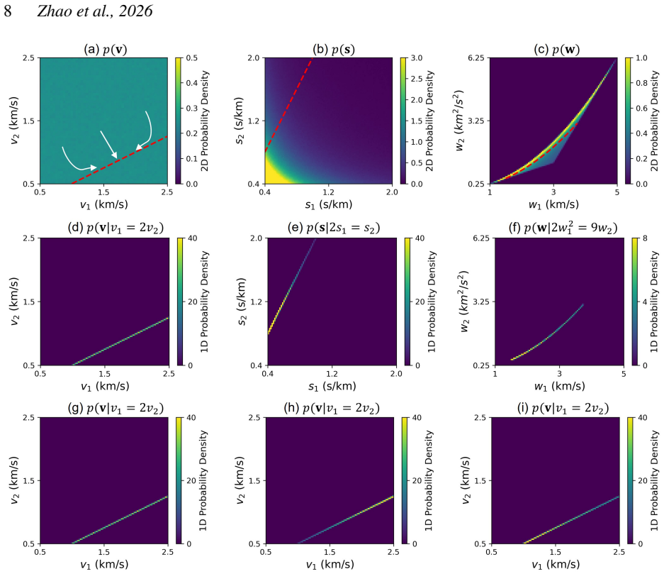
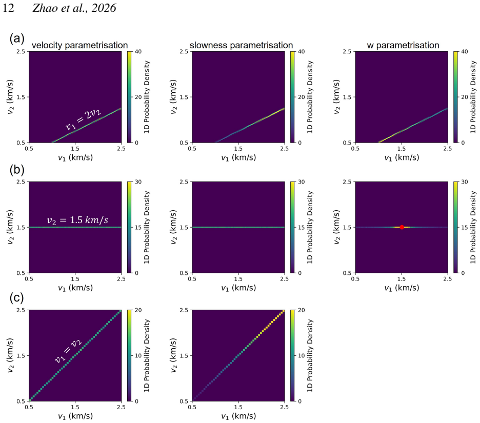
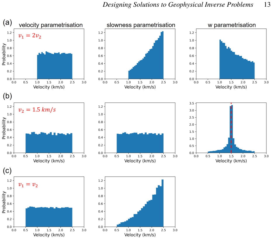
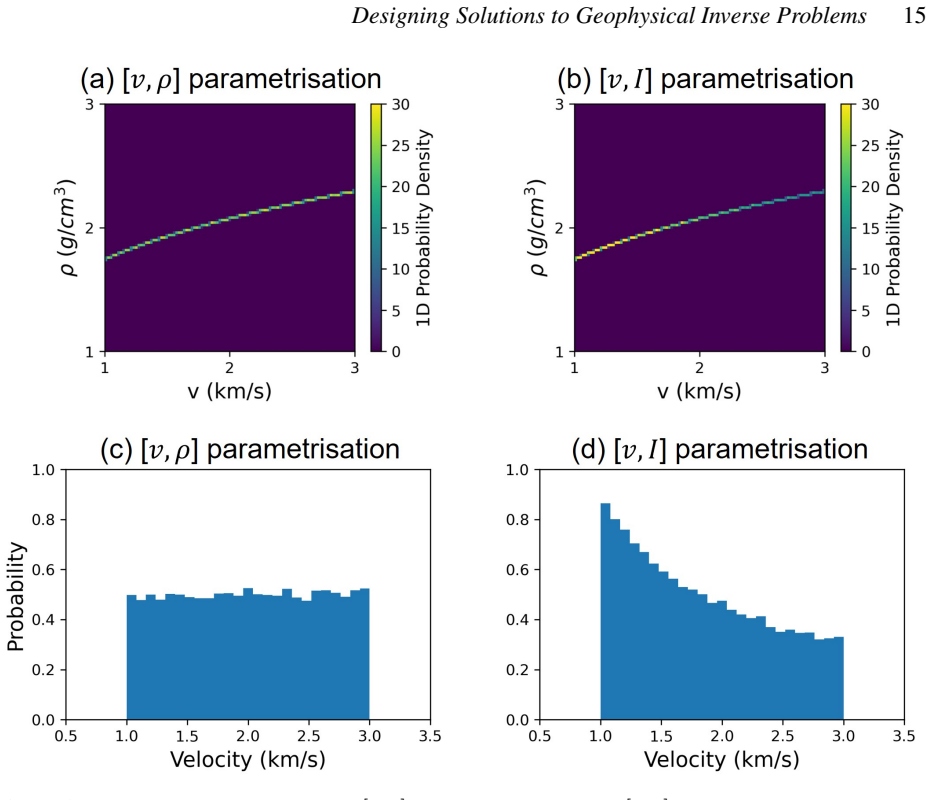
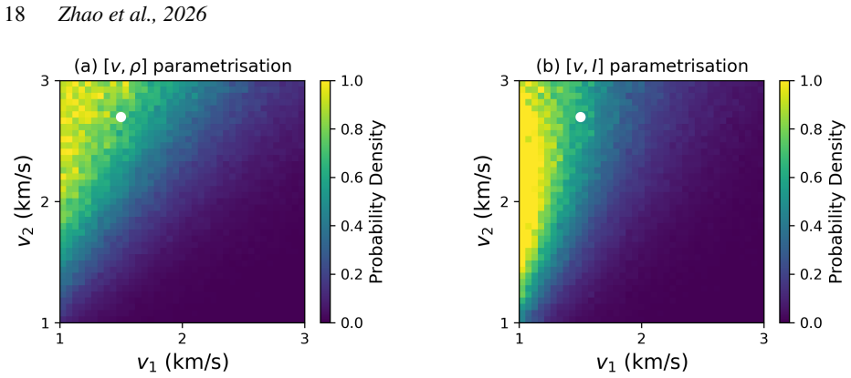
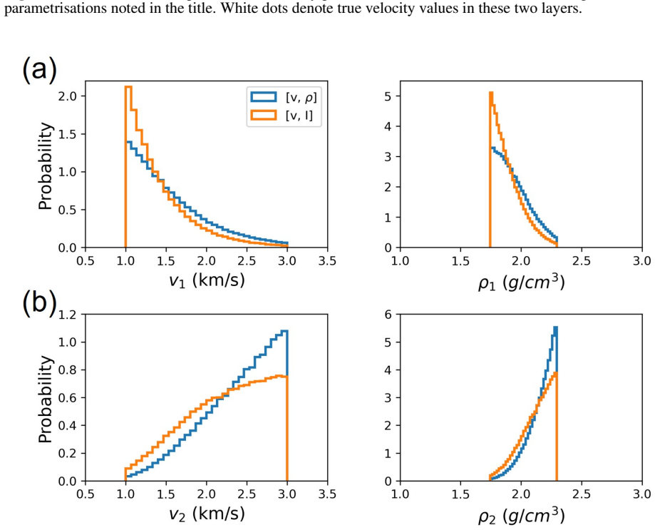
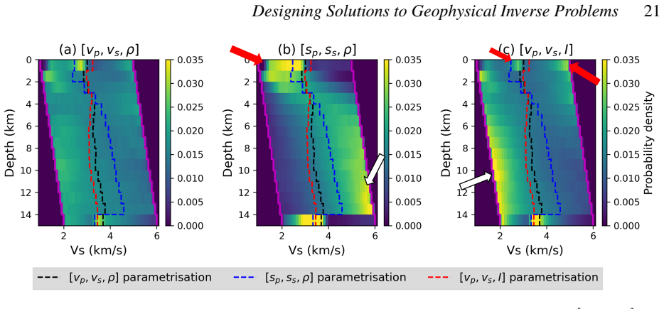
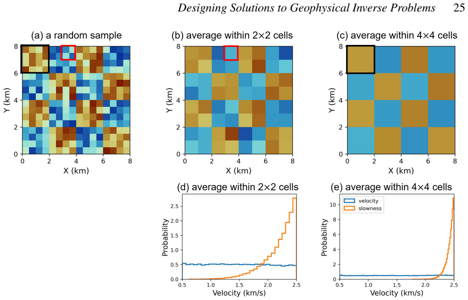
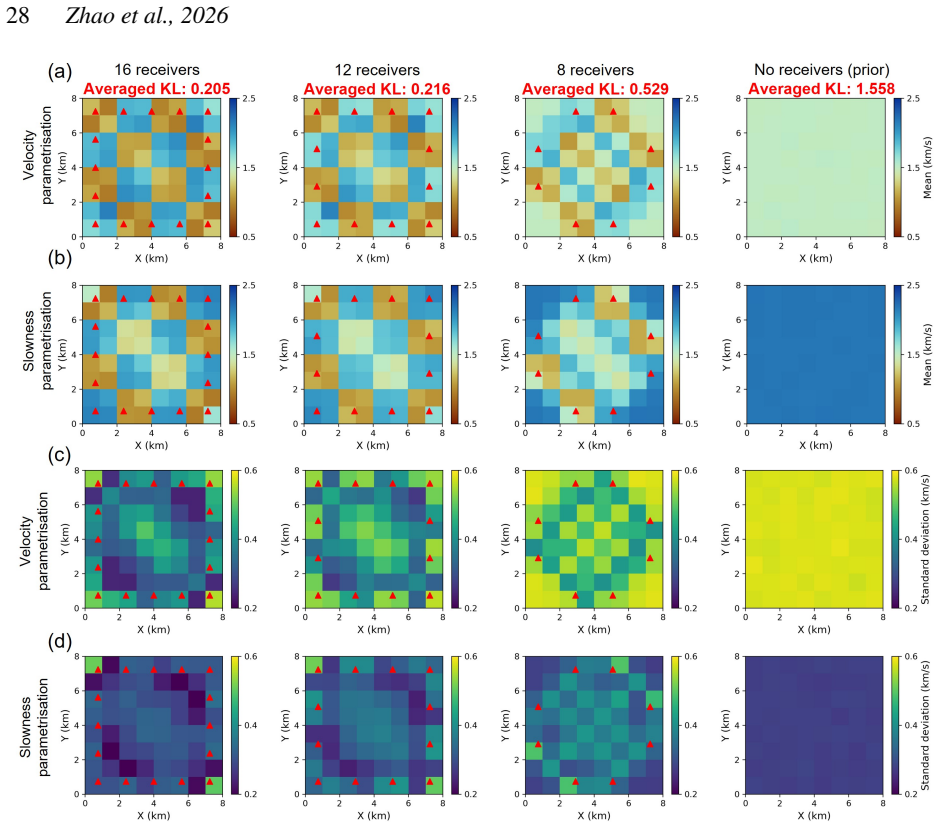
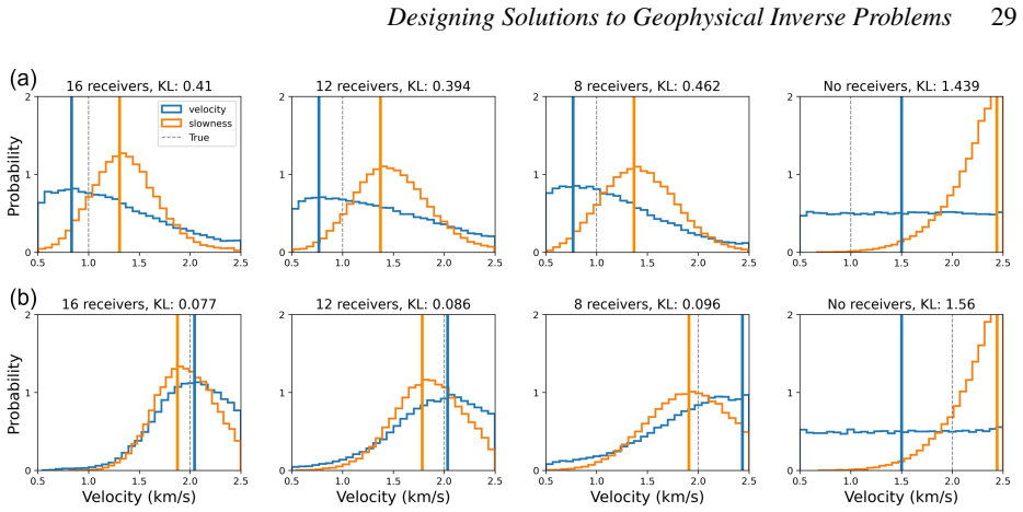
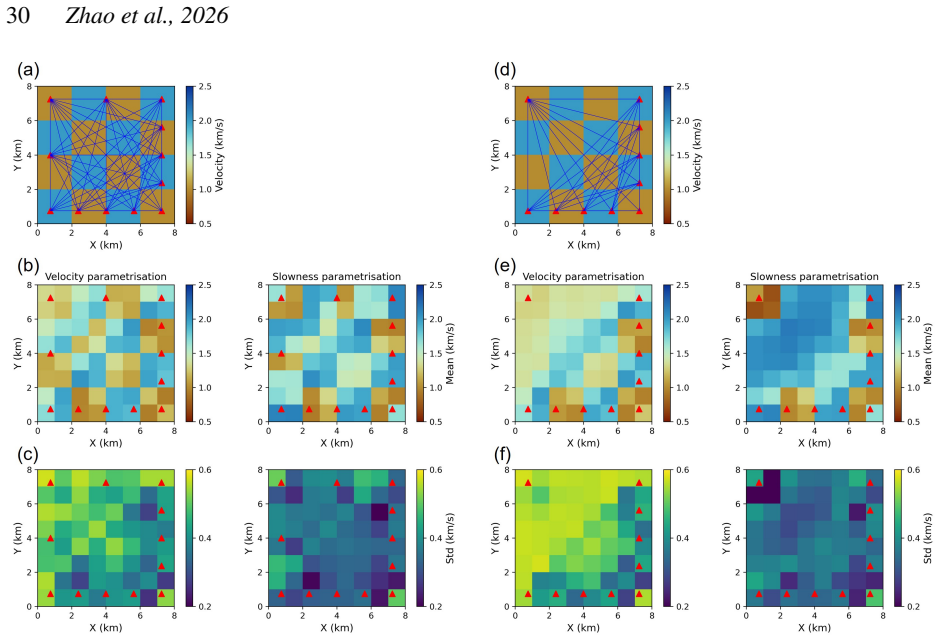
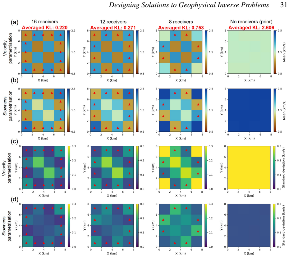
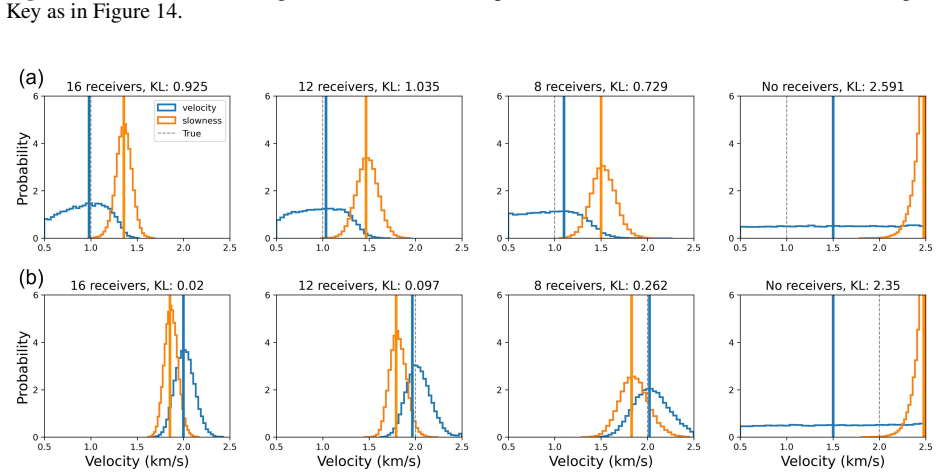
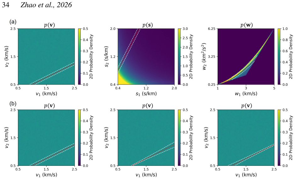
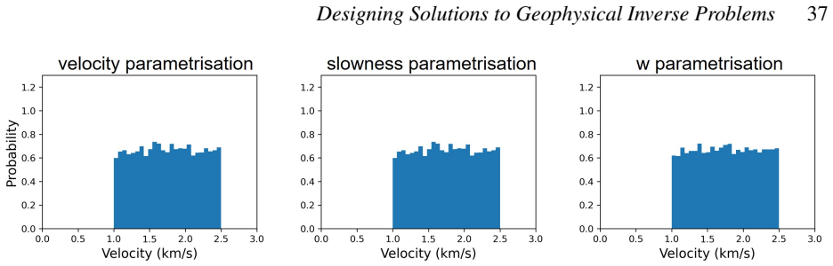
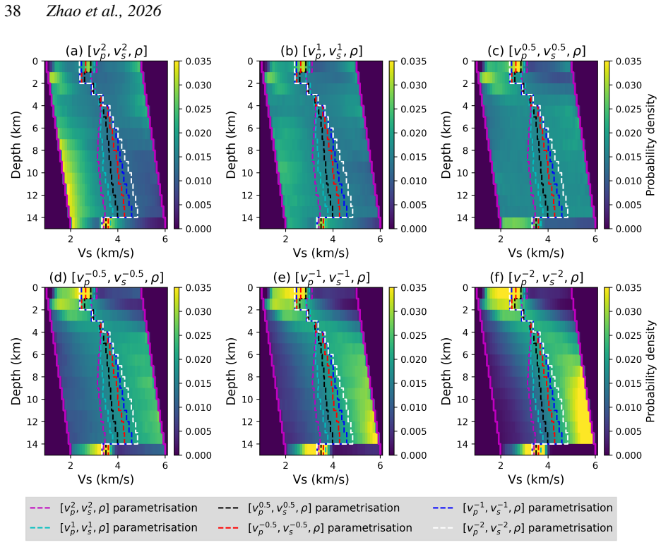
Different parametrisations that encode exactly the same information yield mathematically inconsistent conditional probability densities. When these densities are used in Bayesian inference for geophysical inverse problems with real and synthetic data, the resulting posterior solutions differ dramatically. Because deterministic inversion is mathematically equivalent to computing the maximum a posteriori solution, the same inconsistency appears in deterministic results as well. Solutions can therefore be designed simply by changing the parametrisation.

What carries the argument

The BK-inconsistency: the mathematical inconsistency between conditional probability densities obtained from equivalent but differently parametrised descriptions of the same information.

If this is right

Bayesian posterior solutions for geophysical problems differ dramatically depending on the chosen parametrisation.
Deterministic inversion results become inconsistent across parametrisations because they match maximum a posteriori solutions.
Solutions to inverse problems can be designed or steered by selecting appropriate parameter representations.
A rethinking of Bayesian inference and deterministic inversion may be required for physical problems.

Where Pith is reading between the lines

These are editorial extensions of the paper, not claims the author makes directly.

Uncertainty estimates used for risk-based decisions may depend on the arbitrary choice of variables rather than being unique to the data.
Consistency checks across multiple equivalent parametrisations could become a standard validation step in geophysical workflows.
The effect may extend to inverse problems outside geophysics whenever Bayesian or MAP-based methods are applied to continuous parameters.

Load-bearing premise

That different parametrisations truly encode exactly the same information and that observed differences arise solely from the BK-inconsistency rather than implementation details or data-specific choices.

What would settle it

Apply two equivalent parametrisations to the same geophysical data set and prior information, then check whether the resulting posterior probability densities and deterministic inversion solutions are identical.

Figures

Figures reproduced from arXiv: 2604.26937 by Andrew Curtis, Klaus Mosegaard, Xuebin Zhao.

**Figure 1.** Figure 1: Probability density functions (pdf’s) of the same 2D uniform prior distribution defined for a velocity random variable v, represented by three different parametrisations: (a) velocity v, (b) slowness s, and (c) w. Dashed red lines illustrate a parameter subspace manifold defined by a condition v1 = 2v2 (and equivalently 2s1 = s2; 2w 2 1 = 9w2). White arrows in (a) exemplify different ways to approach the … view at source ↗

**Figure 2.** Figure 2: Conditional pdf’s of velocity parameters along manifold subspace: (a) v1 = 2v2, (b) v2 = 1.5 km/s, and (c) v1 = v2. From left to right, each column displays the results obtained using one particular parametrisation. Note that p(w) does not have valid definition given v1 = v2, therefore we leave this panel blank. Red dot in the right panel in (b) denotes a singular point of p(w) given v1 = v2 = 1.5 km/s. B… view at source ↗

**Figure 3.** Figure 3: Conditional marginal pdf’s of parameter v1, corresponding to the results shown in view at source ↗

**Figure 4.** Figure 4: Prior pdf’s evaluated under (a) [v, ρ] parametrisation and (b) [v, I] parametrisation, conditioned on the Gardner’s empirical relation in equation 8. (c) and (d) are the corresponding marginal pdf’s of P-wave velocity v. coefficient of the interface between the layers. The forward function that estimates the seismic reflection coefficient r for waves arriving at normal incidence to the surface, given the s… view at source ↗

**Figure 5.** Figure 5: Conditional posterior pdf’s of [v, ρ] parameters in the bottom layer, given fixed values in the top layer, and a single reflectivity datum. Key as in view at source ↗

**Figure 6.** Figure 6: Posterior bivariate pdf’s of two velocity parameters v1 and v2, each obtained using the different parametrisations noted in the title. White dots denote true velocity values in these two layers view at source ↗

**Figure 7.** Figure 7: Posterior marginal pdf’s obtained using two different parametrisations (see legend) for the 4- dimensional reflectivity inversion problem. (a) and (b) represent marginal pdf’s of parameters in the first and second layers, respectively view at source ↗

**Figure 8.** Figure 8: (a) Parametrisation of 15 subsurface layers in the surface wave inversion example. Magenta lines show lower and upper bounds of a uniform prior distribution of vs in each layer. (b) Observed Love wave group velocity dispersion curve at geographical location 55.93◦N latitude and 3.18◦W longitude, near Edinburgh city centre. Error bars show data standard deviations used to define an uncorrelated Gaussian lik… view at source ↗

**Figure 9.** Figure 9: Posterior marginal distributions of shear velocity at each depth, obtained using (a) [vp, vs, ρ], (b) [sp, ss, ρ], and (c) [vp, vs, I] parametrisations. In each panel, dashed lines with different colours display the posterior mean models from different parametrisations. At depths beyond 4 km, the posterior marginal pdf’s are biased towards high vs in Figure 9b, and are biased towards low vs in Figure 9c, c… view at source ↗

**Figure 10.** Figure 10: Observed Love wave dispersion curve (red line) and modelled ones (grey lines) obtained using posterior samples obtained from different parametrisations. left red arrow in Figure 9c (at low vs values), and are slightly higher around the right red arrow (at high vs values), compared to those in Figure 9a. Although the trade-off in Figure 9c is subtle, it is robust in multiple independent McMC runs. We also … view at source ↗

**Figure 11.** Figure 11: Posterior marginal distributions of shear velocity at each depth, obtained using (a) [vp, vs, ρ], (b) [sp, ss, ρ], and (c) [vp, vs, I] parametrisations, without applying the inter-parameter relations. In each panel, dashed lines with different colours display the posterior mean models from different parametrisations. model sample from the Monte Carlo algorithm represents a valid solid Earth structure. Not… view at source ↗

**Figure 12.** Figure 12: True velocity model used in a travel time tomography example. Low and high velocity values are 1 km/s and 2 km/s, respectively. Dashed black lines show a discretisation of the true velocity model into a grid of 16 × 16 cells. White and black crosses mark two locations whose posterior marginal distributions are compared in Figures 15 and 18. accurate and provides what we will refer to as high resolution re… view at source ↗

**Figure 13.** Figure 13: (a) A random model sample from the prior pdf. (b) and (c) Samples obtained by averaging parameter values in (a) within 2 × 2 or 4 × 4 cells, respectively, as illustrated by red and black square outlines. (d) and (e) Conditional marginal histograms of velocity values in one arbitrary cell evaluated under velocity and slowness parametrisations. be used to build an unbiased Monte Carlo estimator under the or… view at source ↗

**Figure 14.** Figure 14: All of the features in Figures 14 and 15 prove that the degree of posterior inconsistency view at source ↗

**Figure 14.** Figure 14: Posterior mean velocity maps given the condition that parameter values within 2 × 2 cells are averaged, using (a) velocity and (b) slowness parametrisations, respectively. (c) and (d) Posterior standard deviation maps corresponding to the mean velocity maps in (a) and (b). From left to right, each column shows the inversion results obtained using 16, 12 and 8 receivers, as well as no receivers on the righ… view at source ↗

**Figure 15.** Figure 15: Posterior marginal pdf’s at locations marked by (a) white cross and (b) black cross in view at source ↗

**Figure 16.** Figure 16: (a) and (d) Two uneven station configurations, with blue lines showing straight ray paths considered for each inversion. (b) and (e) Posterior mean maps obtained using each parametrisation. (c) and (f) Corresponding posterior standard deviation maps. most column with no data), the two sets of posterior marginal pdf’s obtained using the slowness parametrisation (orange histograms) exhibit biases in opposi… view at source ↗

**Figure 17.** Figure 17: Posterior statistics given the condition that parameter values within 4 × 4 cells are averaged. Key as in view at source ↗

**Figure 18.** Figure 18: Posterior marginal pdf’s given the condition that parameter values within 4 × 4 cells are averaged. Key as in view at source ↗

**Figure 19.** Figure 19: (a) 2D pdf’s corresponding to those in Figures 1a, 1b and 1c. Dashed white lines in each panel show two bounds of each interval represented in equation 11. (b) Corresponding results after transforming the pdf’s back to the velocity parametrisation. Dashed white lines show the two bounds in equation 12. area between the two dashed white lines in each case represents the 1D conditional pdf given the conditi… view at source ↗

**Figure 20.** Figure 20: Condition marginal pdf’s of parameter v1 given the condition v1 = 2v2 evaluated from three different parametrisations. (a), (b) and (c) represent the results evaluated by approaching the manifold subspace linearly through v1 = 2v2, reciprocally through 2/v1 = 1/v2 and quadratically through v 2 1 = 4v 2 2 . Note that panel (a) and Figure 3a display the same results. For better comparison, orange histogram… view at source ↗

**Figure 21.** Figure 21: Condition marginal pdf’s evaluated by approaching the manifold subspace (v1 = 2v2) along particular directions (a) v1 = 2v2, (b) 1/s1 = 2/s2 and (c) w1 ± p w2 1 − 4w2 2 = w1 ∓ p w2 1 − 4w2 (equation 16) that provide consistent probabilistic results. the unknown model parameter v = [v1, v2] T . The forward problem is defined as d = v1−2v2 which calculates the difference between the first parameter value an… view at source ↗

**Figure 22.** Figure 22: Posterior marginal distributions of shear velocity over depth, obtained using 6 different but equivalent parametrisations. In each panel, identical dashed lines with different colours display the posterior mean models from the six parametrisations. Bodin et al. 2012b; Galetti & Curtis 2018; Zhang et al. 2018) and hierarchical Bayesian inversion (Malinverno & Briggs 2004; Bodin et al. 2012a) are commonly u… view at source ↗

read the original abstract

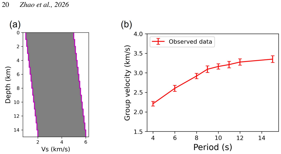
Geoscientists often solve inverse problems to estimate values of parameters of interest given relevant data sets. Bayesian inference solves these problems by combining probability distributions that describe uncertainties in both observations and unknown parameters, and we require that the solution provides unbiased uncertainty estimates in order to inform risk-based decisions. It has been known for over a century that employing different, but equivalent parametrisations of the same information can yield conditional probabilities that are mathematically inconsistent, a property referred to as the BK-inconsistency. Recently this inconsistency was shown to invalidate the solutions to physical problems found using several well-established methods of Bayesian inference. In this study, we explore the extent to which this inconsistency affects solutions to common geophysical problems. We demonstrate that changes in parametrisations result in inconsistent conditional probability densities, even though they represent exactly the same information. We show that this can affect Bayesian posterior solutions dramatically across various geoscientific problems using real and synthetic data. Given that deterministic inversion is often equivalent to finding the maximum a posteriori solution to specific Bayesian problems (the mathematical equations to be solved are identical), the BK-inconsistency also results in inconsistent solutions to deterministic inverse problems. Indeed, we show that solutions can potentially be designed, simply by changing the parametrisation. This study highlights that a careful rethinking of Bayesian inference and deterministic inversion may be required in physical problems: the effects that we demonstrate are likely to affect past and present inverse problem solutions in a variety of different fields of application.

Editorial analysis

A structured set of objections, weighed in public.

Desk editor's note, referee report, simulated authors' rebuttal, and a circularity audit. Tearing a paper down is the easy half of reading it; the pith above is the substance, this is the friction.

Desk Editor's Note private letter to a colleague

The paper applies the known BK-inconsistency to geophysics and shows large posterior shifts on real and synthetic data, but the equivalence claim needs explicit Jacobian checks on the priors.

read the letter

The main thing to know is that this work takes the century-old BK-inconsistency and tests whether it produces big practical differences in common geophysical inverse problems. They report that switching parametrizations changes the conditional densities and posteriors dramatically even when the underlying information is supposed to be identical, and they extend the point to deterministic MAP solutions since the equations match. The real-data examples give the claim some grounding beyond theory alone.

Referee Report

2 major / 3 minor

Summary. The paper claims that the Bertrand-Kolmogorov (BK) inconsistency implies that distinct but equivalent parametrizations of the same geophysical information produce mathematically inconsistent conditional probability densities. It reports empirical demonstrations of dramatic effects on Bayesian posterior solutions across common geoscientific inverse problems (real and synthetic data), notes that deterministic inversion is equivalent to MAP estimation and is therefore also affected, and concludes that solutions can be 'designed' simply by changing the parametrization, necessitating a rethinking of Bayesian and deterministic methods in physical problems.

Significance. If the demonstrations establish that the compared parametrizations induce identical measures on the underlying physical space, the result would be significant: it would show that a known but under-appreciated inconsistency can produce practically large changes in geophysical inversions, offering both a diagnostic and a constructive route to solution design. The empirical scope across multiple problems strengthens the case for re-examination of standard practices.

major comments (2)

[Abstract; demonstrations (real/synthetic examples)] The central claim requires that the two parametrizations encode exactly the same information, which in continuous settings demands that the prior density in the second parametrization equals the first density multiplied by the absolute Jacobian determinant of the coordinate transformation. The abstract and demonstrations assert equivalence without reference to this transformation; if the priors are instead chosen independently or ad-hoc in each coordinate system, the reported posterior differences are explained by mismatched measures rather than by BK-inconsistency.
[Demonstrations section] To isolate the BK-inconsistency as the load-bearing mechanism, the paper must show that the conditional densities differ even after the priors have been properly transformed. Without an explicit Jacobian check or equivalent measure-preserving construction in the examples, the dramatic effects cannot be attributed to the claimed source and may instead reflect implementation details or data-specific prior choices.

minor comments (3)

[Abstract] The abstract states that the BK-inconsistency has been 'known for over a century'; add a specific citation to the original Bertrand or Kolmogorov statements and to the recent work that showed it invalidates certain Bayesian methods.
[Introduction / Methods] Notation for conditional densities should be clarified when changing variables; e.g., distinguish p(m|d) from p(m'(d)|d) and indicate whether densities are with respect to Lebesgue measure in each coordinate system.
[Results] Figures showing posterior densities or MAP solutions for different parametrizations would benefit from side-by-side panels with identical color scales and explicit statement of the prior used in each case.

Simulated Author's Rebuttal

2 responses · 1 unresolved

We thank the referee for the careful reading of our manuscript and the constructive comments, which help clarify the conditions under which the reported effects can be attributed to the BK-inconsistency. We respond to each major comment below and will revise the manuscript accordingly to strengthen the presentation.

read point-by-point responses

Referee: [Abstract; demonstrations (real/synthetic examples)] The central claim requires that the two parametrizations encode exactly the same information, which in continuous settings demands that the prior density in the second parametrization equals the first density multiplied by the absolute Jacobian determinant of the coordinate transformation. The abstract and demonstrations assert equivalence without reference to this transformation; if the priors are instead chosen independently or ad-hoc in each coordinate system, the reported posterior differences are explained by mismatched measures rather than by BK-inconsistency.

Authors: We agree that equivalence of information in continuous spaces requires the prior in the transformed parametrization to be the original prior multiplied by the absolute Jacobian determinant. The original manuscript asserted equivalence in the abstract and demonstrations without explicit reference to this transformation or Jacobian verification. This leaves open the possibility that observed differences arise from ad-hoc prior choices rather than the BK-inconsistency. In the revised manuscript we will update the abstract to qualify the equivalence claim and add an explicit discussion of the Jacobian in the demonstrations section, including verification that the priors induce identical measures on the underlying physical space where possible. We will also distinguish between the transformed (measure-preserving) case and the common practical case of independent prior assignment in each parametrization, which our original examples largely reflected. revision: yes
Referee: [Demonstrations section] To isolate the BK-inconsistency as the load-bearing mechanism, the paper must show that the conditional densities differ even after the priors have been properly transformed. Without an explicit Jacobian check or equivalent measure-preserving construction in the examples, the dramatic effects cannot be attributed to the claimed source and may instead reflect implementation details or data-specific prior choices.

Authors: We will revise the demonstrations to include explicit Jacobian checks and at least one measure-preserving construction to verify that the priors encode identical information. This will allow clearer isolation of the BK-inconsistency. In the original examples the priors were assigned according to standard geophysical practice in the chosen parametrization; the dramatic effects therefore illustrate the practical consequences of the inconsistency. The revision will present the properly transformed case alongside the untransformed case to show when the underlying measures agree and when the reported posteriors (and deterministic MAP solutions) diverge. revision: yes

standing simulated objections not resolved

Demonstrating that conditional densities differ after the priors have been properly transformed via the Jacobian would contradict the premise that the parametrizations encode identical information; we can only show consistency of the probability measures in that case while highlighting the practical divergence that occurs without the transformation.

Circularity Check

0 steps flagged

No significant circularity; applies externally known BK-inconsistency to geophysical problems

full rationale

The paper invokes the BK-inconsistency as a property known for over a century and recently demonstrated to invalidate certain Bayesian solutions in physical problems, treating it as an external mathematical fact rather than deriving it from quantities internal to this work. Demonstrations on real and synthetic geophysical data show effects on conditional densities and posteriors when changing parametrisations, with the claim that solutions can be designed via parametrisation change presented as a direct consequence of this external property. No load-bearing steps reduce by construction to the paper's own inputs: there are no self-definitional relations, fitted parameters renamed as predictions, self-citation chains justifying uniqueness, or ansatzes smuggled via citation. The derivation remains self-contained against external benchmarks, with empirical examples providing independent content.

Axiom & Free-Parameter Ledger

0 free parameters · 1 axioms · 0 invented entities

The central claim rests on the externally established BK-inconsistency together with the assumption that the demonstrated examples are representative of common geophysical practice; no new free parameters or invented entities are introduced.

axioms (1)

domain assumption Bayesian inference combines prior and likelihood distributions to obtain a posterior that quantifies uncertainty
Standard premise of the field invoked throughout the abstract

pith-pipeline@v0.9.0 · 5554 in / 1170 out tokens · 26379 ms · 2026-05-07T08:57:33.316555+00:00 · methodology

discussion (0)

Reference graph

Works this paper leans on

12 extracted references · 8 canonical work pages · 1 internal anchor

[1]

Arnold, R

Analyzing inverse problems with invertible neural networks, arXiv preprint arXiv:1808.04730. Arnold, R. & Curtis, A.,

work page arXiv
[2]

Berger, J

Numerical applications of a formalism for geophysical inverse problems, Geophysical Journal International, 13(1-3), 247–276. Berger, J. O., 2013.Statistical decision theory and Bayesian analysis, Springer Science & Business Media. Bernardo, J. M. & Rueda, R.,

2013
[3]

Bloem, H., Curtis, A., & Tetzlaff, D.,

Transdimensional 2D full-waveform inversion and uncertainty estimation, arXiv preprint arXiv:2201.09334. Bloem, H., Curtis, A., & Tetzlaff, D.,

work page arXiv
[4]

44 Zhao et al., 2026 Curtis, A.,

GLAD-M35: a joint P and S global tomographic model with uncertainty quantification, Geophysical Journal International, 239(1), 478–502. 44 Zhao et al., 2026 Curtis, A.,

2026
[5]

Goodfellow, I., Pouget-Abadie, J., Mirza, M., Xu, B., Warde-Farley, D., Ozair, S., Courville, A., & Bengio, Y .,

Pooling methods in deep neural networks, a review, arXiv preprint arXiv:2009.07485. Goodfellow, I., Pouget-Abadie, J., Mirza, M., Xu, B., Warde-Farley, D., Ozair, S., Courville, A., & Bengio, Y .,

work page arXiv 2009
[6]

Hosseini, K., Sigloch, K., Tsekhmistrenko, M., Zaheri, A., Nissen-Meyer, T., & Igel, H.,

Deep decoder: Concise image representations from untrained non- convolutional networks, arXiv preprint arXiv:1810.03982. Hosseini, K., Sigloch, K., Tsekhmistrenko, M., Zaheri, A., Nissen-Meyer, T., & Igel, H.,

work page arXiv
[7]

Auto-Encoding Variational Bayes

Auto-encoding variational Bayes, arXiv preprint arXiv:1312.6114. Koelemeijer, P., Ritsema, J., Deuss, A., & Van Heijst, H.-J.,

work page internal anchor Pith review arXiv
[8]

46 Zhao et al., 2026 Lindseth, R

Diffusioninv: Prior-enhanced bayesian full waveform inversion using diffusion models, arXiv preprint arXiv:2505.03138. 46 Zhao et al., 2026 Lindseth, R. O.,

work page arXiv 2026
[9]

Malinverno, A.,

BayesBay: a versatile Bayesian inversion framework written in Python, Seismological Research Letters, 96(3), 2052–2064. Malinverno, A.,

2052
[10]

Mosegaard, A

Inconsistency and acausality in Bayesian inference for physical prob- lems, arXiv preprint arXiv:2411.13570. Mosegaard, K. & Hansen, T. M.,

work page arXiv
[11]

& Woodhouse, J

48 Zhao et al., 2026 Trampert, J. & Woodhouse, J. H.,

2026
[12]

1-D, 2-D, and 3-D Monte Carlo ambient Designing Solutions to Geophysical Inverse Problems 49 noise tomography using a dense passive seismic array installed on the North Sea seabed, Journal of Geophysical Research: Solid Earth, 125(2), e2019JB018552. Zhao, X. & Curtis, A., 2024a. Physically structured variational inference for Bayesian full waveform invers...

work page arXiv